Sliding baselines and shuffling species: implications of climate change for marine conservation
Abstract
The concept of shifting or sliding baselines refers to the way that significant changes to an ecological system are mistakenly measured against a previous baseline, which may be significantly different from the original state of the system. The concept assumes an ‘original state’ exists and that a return to that state might be possible, if it could be determined and there was sufficient control of human interference. The concept has been important in both marine conservation planning and fisheries management. However, long periods of exploitation, observed and projected climate change, and the disappearance of some environments, suggest that a return to an original state is unlikely to be achievable in many systems. In addition, protection based on static marine protected areas is unlikely to meet common conservation objectives, as species and habitats are moving and species assemblages shuffling with the changing climate. An alternative to modeling single species distribution changes is to examine change in environmental proxies, such as sea surface temperature (SST). Here, projected changes in SST for the period 2063–2065 from a downscaled ocean model are used to illustrate the similarity to, and movements of, present pelagic environments within conservation planning areas off Eastern Australia. The future environment of small planning areas differs from their present environment and static protected areas might not protect range-changing species. Climate-aware conservation planning should consider the use of mobile protected areas to afford protection to species’ changing their distribution, and develop conservation objectives that are not underpinned by a return to historical baselines.
Introduction
The concept of shifting or sliding baselines refers to the way that significant changes to a system are measured against previous baselines, which themselves are significantly different from the original state of the system (Pauly 1995; Pinnegar & Engelhard 2008). The term was popularised by Pauly (1995) in reference to fisheries management where scientists sometimes fail to identify the correct ‘baseline’ population size (e.g. how abundant a fish species population was before human exploitation) and thus work with a shifted baseline when evaluating carrying capacity or previous state. Pauly (1995) provided examples of radically depleted fisheries that were evaluated by experts who used the state of the fishery at the start of their careers as the baseline, rather than the fishery in its ‘pristine’ state. Areas in which a species was abundant hundreds of years ago may have experienced decline over that whole time, but ‘incorrectly’ the population status in recent past decades was considered the appropriate reference point for current population management. In this way large declines in ecosystems or species over long periods of time were masked. This loss of perception of change occurs when each generation redefines what is ‘pristine’.
The shifting baseline concept was further refined and applied to the ecology of kelp forests by Dayton et al. (1998), who noted that changes in species composition and oceanographic variability and regime shifts, coupled with the need for long time series, made it difficult to define quantitative baselines. The baseline concept has an ‘original status’ or equilibrium state as an implicit assumption, with a return to that state considered possible, if it could be determined correctly and there was sufficient control of human interference. Although Dayton et al. (1998) identified that shifts in the oceanographic climate can impact ecological communities for long periods, and hence baselines might be difficult to define, the concept of a former equilibrium state became entrenched in ecological thinking. In the subsequent decades, the baseline concept has become an important one in both fisheries science and marine ecology (Saenz-Arroyo et al. 2005) and is widely reported in the published literature (Fig. 1). As a result, significant and important efforts have been made to reconstruct that past history around the world (Steele & Schumacher 2000; Jackson 2001; Pitcher 2001; Decker & O’Dor 2003) to establish non-exploitation biomass levels (see Pinnegar & Engelhard 2008), and to support the establishment of marine protected areas (Jackson 2001; Pitcher 2001; Worm et al. 2006) such that the past can be recovered. The value of static place-based traditional conservation efforts might need to be reevaluated, however, given the magnitude of historical change over long periods of time (Pinnegar & Engelhard 2008), subsequent changes in ecological processes (see Pitcher 2001) and observed and projected climate change resulting in novel climates (Williams et al. 2007). Consideration of the impact of climate change for the shifting baseline paradigm has lagged, but recent publication trends suggest most researchers are now including at least discussion of complications to the baseline concept (Fig. 1).
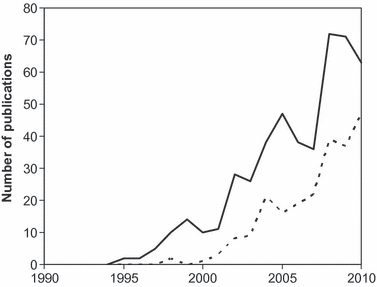
Trend in the number of publications from 1990 to 2010 using the phrase ‘shifting baseline’ (solid line) and ‘shifting baseline’ plus ‘climate change’ (dotted line) using Google Scholar and removing duplicate records (15 January 2011).
Despite evidence of increasing atmospheric greenhouse gas concentrations, particularly carbon dioxide (CO2), since the 1970s (http://scrippsco2.ucsd.edu/), it was not till the late 1990s that scientific consensus for global warming emerged. In 2007, the IPCC stated that warming of the climate system is unequivocal, based on evidence from observations of increases in global average air and ocean temperatures, widespread melting of snow and ice, and rising global average sea level (IPCC 2007). In the ocean, warming and dissolution of CO2 represent a double impact relative to terrestrial systems, and suggest that marine baselines are likely to become an increasingly distant point in history.
Increased concentrations of CO2 in the atmosphere ultimately drive increased uptake by the ocean. The ocean has absorbed about half of the human CO2 emissions into the atmosphere since 1750 (Sabine et al. 2004), leading to acidification of ocean waters. This direct effect of increased CO2 in turn alters the carbonate balance of the oceans and occurs largely independently of anthropogenic global warming (Orr et al. 2005; McNeil & Matear 2008). When CO2 dissolves in seawater it reacts to form weak carbonic acid; oceans are now more acidic than at any time during at least the last 800,000 years (Luthi et al. 2008). Impacts of ocean acidity on a range of species in all oceans have been documented (Orr et al. 2005; Hoegh-Guldberg et al. 2007; Anthony et al. 2008) and major shifts in the capacity for carbonate utilization are projected within several decades (McNeil & Matear 2008).
The second consequence of anthropogenic emission of greenhouse gases is global warming. The rate of warming accelerated in the last decades of the 20th century (Rahmstorf et al. 2007; Le Quéréet al. 2009) and may accelerate further during the 21st century (Schneider 2009). Global oceans have warmed over the last 100 years by an average of approximately 0.6 °C (IPCC 2007), however, ocean temperatures are not increasing homogeneously and the rate of change varies regionally, with some areas warming less rapidly (Alory et al. 2007; Belkin 2009; A.J. Hobday & G.T. Pecl, unpublished data). In Australia, for example, west coast waters are warming around twice as fast as the global average, while warming off Southeast Australia is about four times the global average (Hobday et al. 2007; Ridgway 2007). Within small regions, minor cooling may also occur; for example, increased wind over the coastal ocean can lead to cooling via upwelling (Bakun 1990). Such regional variation is also projected in future (Keenlyside et al. 2008). This variation means that species’ responses may also vary regionally. Oxygen minimum zones and anoxic zones impact on the distribution of many pelagic species (Prince & Goodyear 2006; Rosa & Seibel 2008). Further expansion of oxygen minimum zones is projected in the future (Keeling et al. 2010) which will also impact pelagic species that occupy these regions (Rosa & Seibel 2008; Prince et al. 2010).
The biological responses to these physical changes include changes to phenology and physiology, distribution and abundance, composition and interactions within communities, and structure and dynamics of communities (Walther et al. 2002; Hobday et al. 2007). Examples of marine impacts consistent with climate change now abound, particularly for changes in distribution (Perry et al. 2005; Nye et al. 2009; Last et al. 2011; Pitt et al. 2010).
Given the impact of climate change on the World’s oceans, we are entering a non-analogue future, where a return to a pristine baseline state becomes impossible because historical physical conditions no longer exist (Williams et al. 2007). Critically, climate change that takes place due to increases in carbon dioxide concentration is largely irreversible for 1000 years after emissions stop (Solomon et al. 2009). Atmospheric temperatures are not projected to drop significantly for at least 1000 years. Thermal expansion of the warming ocean means an irreversible global average sea level rise of at least 0.4–1.0 m if 21st century CO2 concentrations exceed 600 ppm and 0.6–1.9 m if CO2 concentrations exceed 1000 ppm (Solomon et al. 2009). Deoxygenation in waters around the world, associated with global warming, is also projected to continue for at least 1000 years (Keeling et al. 2010). These changes can be minimized by a reduction in future greenhouse gas emissions, but are not easily reversed, suggesting that a return to historical baselines from any point in the past is unlikely.
On land, there is a close correspondence between regions with globally disappearing climates and previously identified biodiversity hotspots (Williams et al. 2007); for these regions, standard conservation solutions (e.g. assisted migration and reserves) may be insufficient to preserve biodiversity. Thus conservation solutions based on traditional ‘preserve and protect’ values may need to be extended to cope with shifting climate zones (Lough 2008), just as dynamic spatial management is being used for some fisheries (Hobday et al. 2010a) and considered for pelagic environments (Game et al. 2009).
In this paper, changes in the physical marine environment of Australia are used to illustrate the shifting baselines and shuffling of marine species that are already occurring, and are projected for the future, as a result of climate change. Rather than using individual species distributions, suitable environmental proxies can be used to track the movements of environments and an example is provided of how such proxies might be used in climate-aware marine bioregional planning in oceanic waters of Australia.
Marine bioregional planning in Australia
Marine bioregional planning in Australia includes development of a network of marine protected areas (MPA) which can protect species, habitats and ecological processes (http://www.environment.gov.au/coasts/mbp). As a result of observed changes in the physical environment and biology around Australia (Hobday et al. 2007, 2008; Johnson & Marshall 2007; Poloczanska et al. 2007), both government and stakeholders have recently recognized the need to consider the potential impacts of future climate change in the marine conservation planning process. This planning includes development of a system of national MPAs in Commonwealth waters (3–200 nm from the coast) in five regions around Australia, using a set of goals and principles (http://www.environment.gov.au/coasts/mbp/publications/general/pubs/goals-nrsmpa.pdf), with the planning process scheduled for completion at the end of 2011.
An intermediate step in developing the MPA system is the identification of Areas for Further Assessment (AFA). These AFAs are large areas that encompass representative examples of the range of biodiversity and ecosystems within each marine region. The AFAs may contain species and habitats of conservation value, and both static benthic and dynamic pelagic features of interest; these are identified through stakeholder consultation and focus subsequent MPA selection. Zoning of the final areas also occurs, with some regions given complete protection, and others with only partial restriction of threatening processes. Given that many of these AFAs encompass oceanic waters, the future distribution of pelagic species in these areas is of particular interest.
Likely climate-related range changes for pelagic species in the Australian region have been modeled for only a limited number of species (Hobday 2010; Hartog et al. 2011). Sensitivity to environmental change will vary between species (Hobday et al. 2007); however, this information is unavailable for the majority of species. In the absence of such information on likely individual species changes, changes in suitable proxies can inform conservation planning. In the case of pelagic environments, water mass properties can be suitable proxies for conservation planning (Hyrenbach et al. 2000; Alpine & Hobday 2007; Game et al. 2009).
The waters around Australia, and indeed elsewhere, can be identified as temporally persistent pelagic environments (water masses; e.g.Condie & Dunn 2006; Hobday et al. 2010b). However, these pelagic environments, with features such as water masses, fronts, eddies and currents, are dynamic in space and time (Hyrenbach et al. 2000; Game et al. 2009; Grantham et al. 2011); this mobility makes it hard to predict present and future coverage of these features within AFAs, compared to say, seamounts or reefs, which are static with regard to location. The distribution of many pelagic species is linked to particular pelagic environments, water masses or features (Worm et al. 2005; Prince & Goodyear 2006; Hartog et al. 2011). These associations are being used to assist management in Australian fisheries, for example bycatch of southern bluefin tuna in the east coast longline fishery (Hobday et al. 2010b).
In terms of defining pelagic habitats useful for climate-change studies, environmental variables should be available from both historical datasets and climate change models (Hobday & Lough in press). At present, temperature is the most generally available variable. In particular, sea surface temperature has been shown to be a suitable predictor of pelagic species density and richness (Worm et al. 2005; Boyce et al. 2008) and the dominant physical factor explaining response to climate change in marine systems (Sherman et al. 2009). In turn, sea surface temperature is strongly correlated with a range of other environmental variables, including salinity, oxygen content, and chlorophyll, although different relationships exist in different regions, and not all subsurface pelagic environments may be well linked to surface features.
Sea surface temperature is used here as a proxy to illustrate future changes in pelagic environments in the East Marine Region of Australia, where eight AFAs have been identified. This region stretches from the tip of Cape York to the far coast of New South Wales, but excludes the Great Barrier Reef and Torres Strait (Fig. 2). These AFAs cover a range of water masses and hence pelagic environments. These water masses will move location under climate change, likely taking their biology, such as pelagic tunas and sharks, with them (Hobday 2010). New water masses may also appear in future, based on new combinations of physical variables, as has been postulated for terrestrial environments (Williams et al. 2007). Thus, these conservation planning units may contain different water masses and biology in future compared to the present.
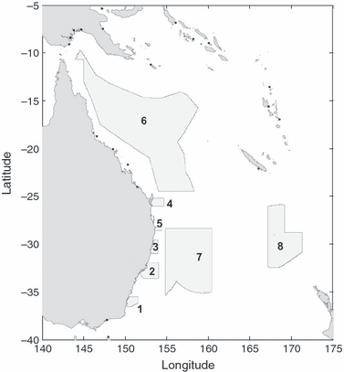
Areas for Further Assessment (AFA) as part of marine conservation planning in the East Marine Region of Australia. 1, Batemans; 2, Hunter; 3, Clarence; 4, Fraser; 5, Tweed; 6, Coral Sea Conservation Zone; 7, Tasmantid – Lord Howe; 8, Norfolk.
Two approaches to assess the difference between the present and future environment found within these AFAs are presented here. In both cases, the environment is represented by sea surface temperature, which is available from both historical datasets and climate change models. The first approach allows an estimate of the pelagic environment that is retained within an individual conservation area, and assumes that protecting a portion of the water mass will also protect the associated species. A high level of retention of the present AFA environment (represented by SST) within the AFA in the future would be desirable. The second approach considers where the pelagic environment (SST) presently contained within an AFA will be found in the future. These results can be used to inform the planning of a network of reserves that will accommodate or even track the shifting environment, and hence offer the potential to protect the species contained with the water mass in the face of climate change. They also serve to illustrate that the baseline concept (Pauly 1995; Dayton et al. 1998), and a return to a former state, should be reevaluated as a conservation planning objective.
Methods
Projected temperatures are available from global climate models; however, the spatial resolution from these models is coarse (1–2°) and is not considered suitable for investigation at the scale of individual AFAs (Hobday & Lough in press). Dynamically downscaled projections using finer resolution models are now becoming available, albeit for a limited number of future scenarios, and represent an opportunity to inform conservation planning at a regional scale (Fig. 3; Hobday & Lough in press). For this study, daily sea surface temperature from the Bluelink ocean model (Oke et al. 2008) nested within the CSIRO Mk3.5 global climate model (GCM), was available for a single historical (1998–1999) and future period (2063–2065) at a spatial scale of 0.1° (∼12 km2; M. Chamberlain, CSIRO Hobart, personal communication). This finer resolution data has previously been used to project the future distribution of southern bluefin tuna and yellowfin tuna (Hartog et al. 2011).
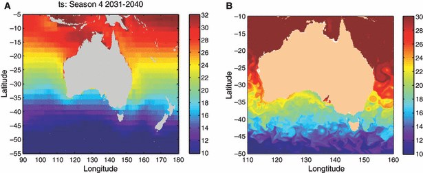
Resolution in projected sea surface temperature (SST). (A) Examples from the CSIRO Mk3.5 global climate model showing projected average SST for spring (months September–November) for the decade 2031–2040. (B) Example of dynamically downscaled SST data, from the Bluelink model nested in the CSIRO global climate model, for the month ‘April 2064’.
Because the future is unknown and can be modified by human responses to climate change, the Intergovernmental Panel on Climate Change (IPCC) developed a set of scenarios for recent IPCC assessments (IPCC 2007). These scenarios represent a range of global warming: low (e.g. SRES BI, CO2 concentration stable at 549 ppm by 2100 and global temperatures approximately 2–4 °C higher); medium (e.g. A1B, CO2 concentration at 717 ppm by 2100 and global temperatures approximately 3–5 °C higher); and high (e.g. A1FI, CO2 concentration at 970 ppm by 2100 and global temperatures approximately 4–6 °C higher). A number of scenarios are often used in projection studies as a way of bracketing the future change, although given present rates of greenhouse gas emission and observed climate change (Rahmstorf et al. 2007; Le Quéréet al. 2009) low scenarios are less realistic. Here only the medium A1B scenario was available using the nested model approach.
Before using future projections, it is important to evaluate whether historical patterns are reproduced when the model is run for the historical period (Hobday & Lough in press). Composite 3-day satellite observations (present period) were available to validate the model. The use of composite dataset reduces the effect of cloud cover, which can result in bias or missing data in individual satellite passes.
The present SST environment within each AFA was first compared for each season using the satellite observations and model output for the historical period (1998–1999). This 2-year period is the length of the historical period available from the nested Bluelink model (M. Chamberlain, CSIRO Hobart, personal communication). The short period of model data is a concern; however, preliminary investigation showed that average SST for each season for each AFA in Eastern Australia calculated using a 2-year time period of satellite data (1998–1999) were similar to values generated using a 5-year time period of satellite data (1998–2002), thus a 2-year period was considered sufficient for comparison with the model data. This short period was not compromised by phases of the ENSO cycle, which often have a minor ocean temperature effect in Eastern Australia (Holbrook et al. 2009). In general, such short periods may not be suitable as ‘typical conditions’ if strong responses to La Nina or El Nino occur.

The second approach involved estimating the upper (5th percentile) and lower SST (95th percentile) values from the present frequency distribution for each AFA and then mapping the distribution of temperatures within this range in the future (2063–2065). This visual result can be used to illustrate to planners and stakeholders the best location for an MPA within an AFA, as well as the value of a network of MPAs.
Results
Comparison between present sea surface temperatures as observed by satellite and model temperatures for the historical period showed that the model values were similar to the observed values (all similarity scores >80%), and so the model was used for historical and future periods to maximize internal consistency. The Bluelink model projects that sea surface temperatures in this region warm by approximately 2° by 2063–2065 relative to the historical period. This is consistent with projections described in previous work using a range of methods (e.g.Hobday et al. 2008; Hobday & Lough in press).
The model projects, based on the medium climate change scenario, that future warming will occur in each AFA in all seasons (Fig. 4). The difference between the two periods of time is illustrated by the dotted line (frequency of present temperature values) and the solid line (frequency of future temperature values). A movement to the right of the future temperature distribution (solid line) indicates warming relative to present conditions (dotted line). Overall, the projected similarity with the present SST environment ranged from 47.6% (Tasmantid) to 1.9% (Fraser; Table 1). There were seasonal differences in similarity scores, which ranged from zero in three of the four seasons for Fraser, to over 50% in winter for the Coral Sea Conservation Zone. Overall, summer (mean 24.6%) and autumn (24.9%) similarities were lower than for winter (30.3% and spring (31.6; Table 1). By 2063–2065, the similarity is <30% for 16 of the 32 season-AFA combinations (Fig. 5). Other values on the tradeoff curve could be used to determine a minimum level of similarity desirable for climate change considerations.
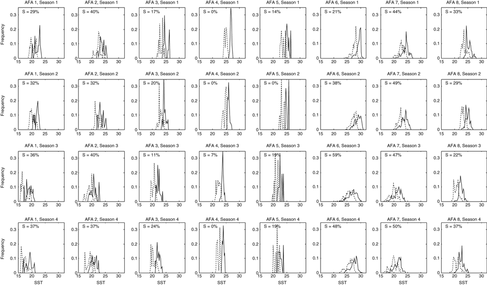
Sea surface temperature distribution within each Area for Further Assessment (AFA; columns 1–8) for each season (row 1–4) for the present (dotted line) and future (solid line). The similarity score (S) is shown in each panel. The AFA regions are, from left to right; 1, Batemans; 2, Hunter; 3, Clarence; 4, Fraser; 5, Tweed; 6, Coral Sea Conservation Zone; 7, Tasmantid – Lord Howe; 8, Norfolk.
| Region | AFA | Summer (% similar) | Autumn (% similar) | Winter (% similar) | Spring (% similar) | Average (% similar) |
|---|---|---|---|---|---|---|
| 1 | Batemans | 28.6 | 31.9 | 36.3 | 37.4 | 33.5 |
| 2 | Hunter | 39.5 | 31.9 | 40.0 | 36.7 | 37.0 |
| 3 | Clarence | 16.9 | 19.7 | 11.3 | 23.9 | 18.0 |
| 4 | Fraser | 0.0 | 0.0 | 7.5 | 0.0 | 1.9 |
| 5 | Tweed | 14.3 | 0.0 | 19.0 | 19.0 | 13.1 |
| 6 | Coral Sea Conservation Zone | 20.8 | 37.8 | 58.9 | 48.3 | 41.5 |
| 7 | Tasmantid | 44.1 | 48.6 | 47.3 | 50.2 | 47.6 |
| 8 | Norfolk | 32.5 | 29.4 | 21.9 | 37.3 | 30.3 |
| Average | 24.6 | 24.9 | 30.3 | 31.6 |
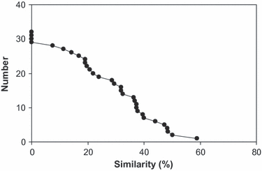
Tradeoff curve illustrating the similarity between historical and future sea surface temperature environments for each AFA-season combination. For example, <10 combinations have more than 40% similarity.
The second approach to inform conservation planning considered the location of the present AFA surface physical environment, represented by SST, by the years 2063–2065. The location of the present SST environment in the future years (2063–2065) was to the south for all the AFAs. For small coastal AFAs, very little of the original pelagic environment is retained within the AFA in the future in any season (Fig. 6A). In larger AFAs, some of the original environment was retained in all seasons by the years 2063–2065 (Fig. 6B).
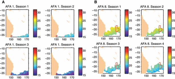
Example of the projected location of the present pelagic AFA environment, as represented by sea surface temperature (see color bar), averaged for each season for the period 2063–2065. (A) Batemans (AFA 1); (B) Norfolk (AFA 8).
Discussion
Climate change has already led to the movement of marine physical environments and species in Eastern Australia (Poloczanska et al. 2007; Ridgway 2007). This is expected to continue into the future for both the physical environment (Hobday & Lough in press) and species (Hobday 2010), which has implications for conservation planning and also questions the utility of the baseline concept (Dayton et al. 1998) for setting conservation goals. Here, two approaches were developed to illustrate the likely future physical surface environment in areas identified for establishing MPAs.
In general, the larger areas with a greater latitudinal range have more overlap between present and future environments (AFA 6, 7, and 8), wheresd areas with a smaller latitudinal range retain less of their present pelagic environment by 2063–2065. The AFAs retaining the least of the present pelagic environment represented by sea surface temperature are the small coastal locations (AFA 3, 4, and 5). Intermediate coverage of the future environment was projected for the remaining AFAs (1 and 2). The projected southward movement of the SST environment demonstrated by the second approach is consistent with historical observations that show warming and southward extension of the East Australia current and southward movement of many marine species and habitats (Poloczanska et al. 2007; Ridgway 2007; Figueira & Booth 2009; Ling et al. 2009; Last et al. 2011; Pitt et al. 2010) and with future projections in other studies (Hobday 2010; Hobday & Lough in press).
To address the impact of future climate change on each AFA as part of the final step in regional marine planning, selection of individual MPAs, results from either approach may be used, as the results are complementary to a point. Obviously, when similarity is high, the movement of habitat will also be low; however, when similarity between present and future environments is low, the second approach is more informative, as it illustrates where and how far the habitat has moved. Both representations could be used to indicate to stakeholders how each of the AFAs would cope with future climate and inform climate-aware reserve design. Other useful summary metrics might include the fraction of present AFA environment located in another AFA in future. If a time series analysis were possible based on climate projections for the complete period (e.g. 1998–2065), calculations of habitat trajectories of change could show the fraction of time each original AFA environment spent outside any AFA. The same analysis could also be completed at the scale of individual MPAs, although treating the MPAs as a network in such analysis would be preferable, due to the smaller size of MPAs relative to AFAs.
A suitable similarity value to ensure that a protected area also meets its conservation objectives in a future period cannot be defined at this time. While modeling studies may be able to determine what is sufficient areal coverage for static or mobile protected areas, setting such thresholds is largely a social or policy decision. Values such as 20% protection of each habitat type (Game et al. 2008) or 30% of a species range have been suggested (Alpine & Hobday 2007), and tradeoff curves can be used to determine a minimum level of similarity desirable for climate change considerations, just as they inform static design (Game et al. 2008). Policy makers and scientists must work to find suitable values for the suite of species and habitats that are to be protected by the MPA, based on their conservation objectives.
This analysis took advantage of the recent completion of a projection for the year 2063–2065 with the Bluelink ocean model nested in a global climate model, under one future climate change scenario (the medium A1B scenario), and a control run for the period 1998–1999. In seeking to compare the present with the future, both the present model years (1998–1999) and the future period (2063–2065) are indicative of each time period and are not intended to represent the specific environment for each set of years. For example, the future year 2063 is assumed to be typical of any year in the period 2060–2065. Other periods might be of interest to conservation planners, such as 2030s or 2100; however, these would have to be addressed using coarser data (raw GCM data; Hobday & Lough in press). Other scenarios and models could also be examined (higher rates of warming, such as the A1FI scenario), to give a range of uncertainty with the projected movements of surface habitats (Hobday 2010). While more dynamically downscaled climate projections might become available, they will not likely to cover the same span of future scenarios as the suite of GCMs used for IPCC assessments, or as statistically downscaled projections (Hobday & Lough in press). In ocean regions where sub-grid scale features such as fronts and eddies are important, only dynamically downscaled models are likely to yield more realistic projections. Thus, there is a tradeoff between scale, and hence process resolution, and scenario variation that must be made when considering climate change as part of conservation planning. The results presented here should be considered with the caveat that they represent just one projected future, and are based on one environmental proxy. Additional model projections would underpin estimates of uncertainty on the rate of habitat movement, while additional variables would allow a more comprehensive description of habitat changes.
A number of physical and biological variables are important in predicting the distribution of pelagic species, including temperature, chlorophyll, oxygen concentration and currents (Worm et al. 2005; Prince & Goodyear 2006; Hobday 2010). Sea surface temperature is commonly used as an indicator of the pelagic environment, as it is widely correlated with the distribution of pelagic species (Sherman et al. 2009) and is available from both present and future model outputs. In addition, this illustrative analysis is representative of surface conditions (∼100 m) rather than the full water column. While general warming is expected at all depths, the rate of warming (and hence southward movement of species) will be slower in subsurface waters (e.g.Alory et al. 2007).
This analysis has demonstrated that the physical environment in Eastern Australian pelagic waters may change relative to historical patterns. Assuming that the species associated with these water masses also move, and historical studies support this assumption (Perry et al. 2005; Greenstein & Pandolfi 2008; Nye et al. 2009; Last et al. 2011), any fixed region will contain a different species mix in future compared to present conditions. However, this movement of species between regions will not be coherent, for several reasons. Species have different tolerances and sensitivities to environmental conditions, including temperature (Worm et al. 2005; Boyce et al. 2008). Species may not be able to keep up with the rate of physical change. Availability of suitable habitat, for example, in a particular depth range, is also a prerequisite for range change. This variation between species movements is evidenced by studies that report a subset of species respond to climate change by changing distribution (Perry et al. 2005; Nye et al. 2009; Last et al. 2011; Pitt et al. 2010). Finally, the change in distribution is fast at the leading edge (e.g. moving poleward) and slow at the receding edge (equator-ward range limit; Perry et al. 2005; Nye et al. 2009; Pitt et al. 2010). Climate change initially leads to an increase in local biodiversity as fast-moving species overtake the slow-moving ones. Thus, the concept of a baseline for planning conservation goals may not be appropriate in the 21st century. However, determining baselines may still be important for referencing how much human activity, even with non-analogue climate change, is modifying marine environments (sensuDayton et al. 1998). A key question is how conservation planning can be improved by an understanding of climate change projections for any particular environment?
Reduction of threats other than climate change is still important, and protected areas have been shown to have positive conservation outcomes in many situations (e.g.Worm et al. 2006). Thus, place-based protection should continue to be important in future. For some features of importance, particularly in offshore regions, dynamic MPAs that track features as they move under climate change should be considered (Hobday et al. 2011). One pelagic long line fishery in Australia has been using such an approach since 2003, with management boundaries regulating fisher access updated every 2 weeks during the fishing season (Hobday et al. 2010a).
There may be legislative or implementation challenges with creating dynamic MPAs (Game et al. 2009; Hobday et al. 2011), in which case static MPAs may still be favored. In the example illustrated in this paper, where environmental change was in a poleward direction, orientation of the long axis of an MPA along the axis of climate movement (latitudinally) is one option; however, this might not cover all species distributed across the longitudinal range of a planning region. Another option would be to locate a MPA in the area of the planning region where the future environment was projected to be most similar to the present environment. In this example, such areas occur in the south of each large AFA, but this is not an option for the small coastal planning regions, where very little of the present environment remained in future. In such cases, a network of MPAs is appropriate. Spacing of these individual areas could be such that some of the environment is contained within at least one MPA at all times for a particular time horizon. Even static MPAs could be modified in time, on a decadal scale, to account for observed changes in ocean environments. Overall, a flexible approach, with a combination of static and mobile MPAs, depending on the species or feature of interest, is recommended given climate change. For example, if seamounts represent a key habitat for some pelagic species, then static reserves are appropriate. If, however, dynamic and moving ocean features such as eddies or thermal ranges represent the habitat for the species of interest, then dynamic (mobile) protected areas may be the best option. Additional work is required to estimate the best size for mobile areas, as many pelagic species are wide ranging, and might only have partial protection during their life.
Conclusion
Protected areas have been recognized as only one tool for species and habitat conservation, and this will be true in future. Fisheries management is embracing adaptive management (Sainsbury et al. 2000; Smith et al. 2007) and, recognizing that, a range of tools should be employed for sustainable management in the face of climate change. Conservation management and planning must also adapt to this new reality, and reformulate conservation goals and practices that are not based on a return to a baseline. The baseline concept may no longer be useful for either fisheries or conservation objectives given climate and other anthropogenic change. In particular, consideration of mobile protected areas should be a part of climate-aware conservation planning. This may require flexible and novel policy – but in a non-analogue, no-baseline future there may be few alternatives.
Acknowledgements
Thank you to the editor Lisa Levin for her invitation to contribute to this special issue in tribute of Paul Dayton. Paul has inspired, and continues to inspire, many people. In particular his encouragement to explore widely, in space, time and thoughts and to consider the practical applications, has helped me to enjoy science as a fulfilling career. I am grateful for his support in my student days, and inspiration since. I also appreciate the collaboration of many colleagues in climate research – such collaboration is critical to minimizing the impact of anthropogenic climate change and to offering future generations an environment they too can love and protect. This work was funded in part by SEWPaC, and advice from Scott Francis and Mandi McKaig in completing parts of this research is appreciated. The Bluelink present and future projections were supplied courtesy of Richard Matear and Ming Feng, supported by the Australian Climate Change Science Program, and they are gratefully acknowledged. The manuscript was improved by comments from the editor and three reviewers.


