Cube law, condition factor and weight–length relationships: history, meta-analysis and recommendations
Summary
This study presents a historical review, a meta-analysis, and recommendations for users about weight–length relationships, condition factors and relative weight equations. The historical review traces the developments of the respective concepts. The meta-analysis explores 3929 weight–length relationships of the type W = aLb for 1773 species of fishes. It shows that 82% of the variance in a plot of log a over b can be explained by allometric versus isometric growth patterns and by different body shapes of the respective species. Across species median b = 3.03 is significantly larger than 3.0, thus indicating a tendency towards slightly positive-allometric growth (increase in relative body thickness or plumpness) in most fishes. The expected range of 2.5 < b < 3.5 is confirmed. Mean estimates of b outside this range are often based on only one or two weight–length relationships per species. However, true cases of strong allometric growth do exist and three examples are given. Within species, a plot of log a vs b can be used to detect outliers in weight–length relationships. An equation to calculate mean condition factors from weight–length relationships is given as Kmean = 100aLb−3. Relative weight Wrm = 100W/(amLbm) can be used for comparing the condition of individuals across populations, where am is the geometric mean of a and bm is the mean of b across all available weight–length relationships for a given species. Twelve recommendations for proper use and presentation of weight–length relationships, condition factors and relative weight are given.
Introduction
Research on weight–length relationships is not considered interesting science by current fisheries scientists. For example, the text book Quantitative Fisheries Stock Assessment (Hilborn and Walters, 2001) expresses this view as follows:
We do not have much to say about length–weight relationships and the allometric growth parameter b. […] Length–weight analysis is a good thing to have your teenage children do as a way of learning about ideas of correlation and regression, and you might find the results mildly useful in estimating average weight of fish caught from samples of lengths of fish caught. If your teenager is having trouble understanding how to estimate b for you, it may be of some comfort to know that you will not likely go far wrong by just assuming b = 3.
In other words, establishing weight–length relationships is considered regular work of the fisheries scientist, with the results typically not meriting publication in scientific journals other than as short communications for species where such relationships were not previously known. On the other hand, as pointed out by Kulbicki et al. (2005), weight–length relationships are only known for a restricted number of species, which hampers efforts to model aquatic ecosystems where observations are typically obtained as the number of specimens by length class that have to be transformed into estimates of the biomass.
Weight–length relationships (WLR) are used for estimating the weight corresponding to a given length, and condition factors are used for comparing the ‘condition’, ‘fatness’, or ‘well-being’ (Tesch, 1968) of fish, based on the assumption that heavier fish of a given length are in better condition. Both concepts have been used in fisheries research since the beginning of the 20th century. They appear simple enough, yet there has been ongoing confusion about their correct interpretation and application. Some of the clarifications and insights summarized in the 1950s are unknown to recent authors. Also, the advent of large compilations of length–weight studies allows revisiting and expanding these insights. This study will thus pursue three aims: firstly, to provide a review of the history of weight–length relationships and condition factor; secondly, to perform a meta-analysis of a compilation of some 4000 length–weight studies for about 2000 species; and thirdly, to provide guidelines for current fisheries workers dealing with length–weight data.
History
 ()
()In an addendum to a report by Hensen (1899), Reibisch (1899) tried to find an indicator for the nutritional condition of plaice Pleuronectes platessa (Linnaeus, 1758) from the Kiel Bight. He divided weight by length and obtained what he called a ‘Längeneinheitsgewicht’ representing mean thickness times mean height, i.e. a kind of mean cross-section of the specimen. However, he found that this new indicator varied with length and weight and did not provide any information that could not be obtained by comparing the weight of specimens of similar length. Following a suggestion by Reibisch, who had to leave Kiel to participate in the evaluation of a German deep-sea expedition, Hensen (1899) also presented what may have been the first publication of condition factors, i.e. individual weights of plaice divided by the cube of the respective length. He found this new measure also to be correlated with length and therefore dismissed it as having no obvious advantage.
Heincke (1908) presented Eqn 1 and credited it to D'Arcy Thompson, without citation. I could not find such a pre-1908 publication by Thompson, i.e. he may have presented it at a meeting or in personal correspondence. Heincke (1908) referred to K as the length–weight coefficient and described two methods for estimation:
- 1
In Eqn 1, take W as the mean weight of all specimens in a given length class, resulting in dedicated estimates of K for every length class (Note that W should be geometric mean weight and L should be geometric mean length of the respective length class, to account for the log-normal distribution of these variables).
- 2
Take W as the total weight of all specimens across all length classes, divided by the sum of all cube lengths. For a given length class this can be expressed as nL3, where n is the number of specimens and L is the (geometric) mean length of the respective length class. This has the advantage of only one determination of weight with a presumably robust balance, a method more suited for work on seagoing vessels. K is then a mean estimate for the respective sample. (This method is not suitable if there is a strong change of condition with length, i.e. if b of the respective WLR is significantly different from 3.)
Heincke (1908) described the seasonal variation of K in plaice of the south-eastern North Sea and found that the better the nutritional condition, the higher is K. He thus established the use of the length–weight coefficient as the ‘Ernährungskoeffizient’ or condition factor. He also realized that differences in condition factor are directly proportional to differences in weight. For example, for autumn plaice he found mean K = 1.04 for males and K = 1.02 for females; for both sexes in spring he found mean K = 0.87 and concluded that, on average, autumn plaice are 16% heavier than spring plaice.
Heincke (1908) developed a special method for measuring the relative muscle thickness of plaice. He found this to be well correlated with the condition factor until the onset of gonad development, when muscle thickness decreased but the condition factor remained about constant, i.e. in plaice some muscle tissue is converted into gonads, as gonad development takes place during winter when feeding intensity is low. Condition dropped abruptly after spawning to K = 0.8 for males and K = 0.7 for females. He concluded that condition of plaice varies with sex, size, season and degree of gonad development. These observations have been confirmed for many other species by subsequent workers such as Crozier and Hecht (1915) for the gray weakfish Cynoscion regalis (Bloch and Schneider, 1801); Thompson (1952, original 1917) for plaice; Menzies (1920) for sea trout Salmo trutta Linnaeus, 1758; Järvi (1920) for the vendace Coregonus albula Linnaeus 1758; Martin (1949) for several North American fishes; Hile (1936) for the cisco Coregonus artedi Lesueur, 1818; Le Cren (1951) for perch Perca fluviatilis Linnaeus, 1758; and most recently several authors (Olim and Borges, 2006, Šantić et al., 2006; Zorica et al., 2006) in this volume for Mediterranean and North Atlantic species. Clark (1928) showed explicitly that the condition factor is highly correlated with fat content in the California sardine Sardinops sagax (Jenyns, 1842), thus confirming Heincke's results for muscle thickness.
Heincke (1908) with his work thus established the correct interpretation of Fulton's condition factor and ‘operationalized’ its application as a standard tool in fisheries management.
Despite the shortcomings already pointed out by Fulton in 1904 and confirmed by subsequent workers, the cube law remained in use in fisheries for estimating weight from length for two more decades. For example, Thompson refers to the correlation between length and weight in the 1917 edition of his book On Growth and Form (here cited from a 1952 reprint of the second edition of 1942), where he presents Eqn 1 for estimating weight from length, and praises its usefulness because it ‘enables us at any time to translate the one magnitude into the other, and (so to speak) to weigh the animal with a measuring-rod; this, however, being always subject to the condition that the animal shall in no way have altered its form, nor its specific gravity.’
Järvi (1920) was the first to realize that a better prediction was obtained if, instead of using the cube, the length-exponent was estimated as a second parameter of the relationship. Järvi (1920) thus published the first modern WLRs, namely W = 0.0050L3.2 for males, W = 0.002 L3.64 for ripe females, and W = 0.0056L3.16 for spent females of vendace in Lake Keitele in Finland. However, he did not explicitly present these equations (he just mentioned the numbers in the text) and did not elaborate on his method of estimation. His work was published in German in Finland and was overlooked by most subsequent workers.
Weymouth (1922), working on the pismo clam Tivela stultorum (Mawe, 1823), also found the cube law to be inaccurate and states:
An exact determination of this relationship, to be treated more in detail elsewhere, shows that the length must be raised to the 3.157 power […], or to express as a formula: weight (in grams) = 0.168 × length3.175.
This may have been the first explicit statement of the WLR equation, but it was overlooked by subsequent workers concerned with fishes.
Duncker (1923) made an effort to improve the prediction of weight from length by applying a third-order polynomial equation of the type W = a0 + a1L + a2L2 + a3L3, where W and L are variables as described above, and a0 to a3 are the four parameters to be estimated. He even applied logarithms to facilitate his calculations, but failed to see that transforming weight and length to logarithms would have allowed fitting a much simpler linear regression, a method well known to biologists of his time. The polynomial equation provided a good fit to the data but was computationally demanding and not adopted by subsequent workers.
Tyurin (1927) used weight-at-length data for the tugun Coregonus tugun (Pallas, 1814) and a variety of other Siberian species to show that when plotted on double-logarithmic paper the points could be fitted with straight lines with similar slopes but different intercepts. He suggested using these graphs for interpolating values for missing observations. However, he failed to realize that the equation describing these straight lines was also the best for predicting weight from length. Instead, he proposed a second-order polynomial equation of the form W = a0 − a1L − a2L2, where W and L are variables as described above, and a0 to a2 are the three parameters to be estimated. His paper was published in Russian and was overlooked by most subsequent workers.
 ()
() ()
()However, shortly after the Keys (1928) paper had been transmitted for publication, i.e. before formal publication, Frances N. Clark (1928) published an extensive paper on The Weight-Length Relationship of the California Sardine, in which she fitted a least-squares regression line to log-transformed weight-at-length data for this species. She presented the modern equation for the relationship and formally declared the cube law to be incorrect for estimating weight from length. Her work was widely noted and from then on Eqn 3 was used by authors to estimate the parameters of the WLR.
However, some confusion resulted as to whether the exponent in Eqn 1 should not be the same as b in the respective WLR, or in other words, whether a = K/100, in which case Fulton's condition factor could have been abandoned. This confusion started with Clark (1928), who used the condition factor to compare relative heaviness in the California sardine, but apparently thought that replacing the cube with the exponent of the respective WLR would have been more accurate. Hile (1936) reviewed the respective publications and found that within a species ‘the values of the coefficient [a] […] depend primarily not on the heaviness of the fish but rather on the value of the exponents. A large value of [b] is associated with a small value of the coefficient [a] – and the reverse.’ He concludes that Fulton's condition factor (Eqn 1) is the appropriate method for comparing relative heaviness, whereas the WLR (Eqn 2) is the appropriate method for estimating weight from length.
 ()
()Hile (1936) presented a first interpretation of the exponent b, namely that the difference from 3.0 indicates the direction and ‘rate of change of form or condition.’ In other words, b < 3.0 indicates a decrease in condition or elongation in form with increase in length, whereas b > 3.0 indicates an increase in condition or increase in height or width with increase in length. The larger the difference from 3.0, the larger the change in condition or form.
Martin (1949) studied the relative growth of body parts and change of form in fishes. He found that while in most species values of the exponent b approximate 3, constant change of form (i.e. b <> 3) is more common than constant form (b = 3). He gave an overview of studies where different WLRs were found for different growth stanzas, typically among larvae, juveniles and adults. He showed that different growth stanzas can be produced experimentally, e.g. by strong changes in water temperature or by starvation.
 ()
()Le Cren (1951) pointed out that the interpretation of the condition factor is difficult and prone to error. For example, a difference in mean condition between two populations can be caused by (i) slight differences in body shape between these populations; (ii) different mean lengths in the respective samples if b <> 3; and (iii) differences in season or development of gonads between the two samples. For perch in Lake Windermere he found that the contribution of gonads to body weight was up to 8% in males and 24% in females. The stomach content contributed up to 2% of body weight, and seasonal deviation from mean body weight was up to 20%.
Le Cren (1951) also compared weight–length relationships for perch in Lake Windermere for different life stages, sexes, stages of gonad development, and different seasons. He found significant differences and concluded ‘that no single regression will adequately describe the length–weight relationship for the perch.’ In particular, he found different growth stanzas and thus WLRs for larvae, age groups 0 and 1, and mature males and females.
 ()
()Ricker (1958) used the term ‘isometric growth’ for ‘the value b = 3 […] as would characterize a fish having an unchanging body form and unchanging specific gravity.’
 ()
()Carlander (1969) published the first volume of his widely used Handbook of Freshwater Biology in which chapters were dedicated to length–weight relationships and to Ponderal Indexes or Condition Factors. He gave equations for converting WLRs if measurements were done in units other than grams and millimetres, such as pounds, inches, or centimetres. He also presented weight-at-length data and relationships for many North American fishes in various water bodies. He showed the first frequency distribution of the exponent b for 398 populations, and found ‘a slight tendency for the slopes to be above 3.0, but the mean is 2.993.’ He examined cases where b was outside the range of 2.5–3.5 and found many of these to be questionable for different reasons. Only ‘five slopes between 3.55 and 3.74 for channel and flathead catfish appear to be valid and related to the tendency for larger catfish to be obviously heavier bodied as they grow.’ He reviewed the relative condition factor (Eqn 5) of Le Cren (1951) and concluded:
While the relative condition factor is useful in certain studies, it is not suitable for comparisons among populations and it assumes that the length–weight relationship remains constant over the period of study.
In the second volume of his handbook, Carlander (1977) showed a plot of log a over b and used it for comparing intercepts (log a) for similar slopes (b) of 41 weight–length relationships of white crappie Pomoxis annularis Rafinesque, 1818 with 75 relationships of black crappies Pomoxis nigromaculatus (Lesueur, 1829). However, he failed to notice the linear relationship between log a and b and its usefulness for detecting outliers among the respective studies (Froese, 2000), such as is glaringly present in his graph.
 ()
()Tesch (1968) used the term ‘allometric growth’ for values other than b = 3. He stated: ‘If b > 3, the fish becomes ‘‘heavier for its length’’ as it grows larger.’
Tesch (1968) also presented a variation of the relative condition factor as ‘allometric condition factor’ CF = w/lb for comparing individual fish. This variant was to be used ‘when a large and representative body of data is available for an allometrically-growing species so that a sufficiently accurate value of b can be computed.’ This proposed variation omits the coefficient a from Le Cren's (1951) calculation of relative condition (Eqn 5). Since a is a constant this gives practically the same results as Eqn 5 (Krel = CF/a), albeit with a non-telling value: while Krel gives the ratio of the observed weight of an individual to the mean weight at this length and thus can be interpreted directly, the value of CF does not lend itself to direct interpretation. Bagenal and Tesch (1978) also presented the CF equation as K′ = 100w/lb and failed to notice that it is basically the same as Eqn 5, which they restated as  , where
  is the geometric mean weight for the respective length derived as anti-log from Eqn 3. The concepts of CF, K′ and K′′ are thus unnecessary and have only led to confusion by subsequent authors. For example, Zorica et al. (2006) show a graph with relative and allometric condition factors, with identical trends and a correlation of 1.00, i.e. the allometric condition factor gives the same information and is thus redundant. Olim and Borges (2006) show seasonal plots of allometric condition, whereas Fulton's condition factor would probably have revealed more pronounced patterns.
Ricker (1973) pointed out that in predictive regressions the resulting regression lines are different depending on whether one predicts Y from X or X from Y. He suggested instead using the geometric mean (GM) functional linear regression, which provides an intermediate line and can be used in both cases. He used weight–length relationships as one example and concluded that ‘Hence the GM line should be used for estimating weight from length, or length from weight.’Carlander (1977) compared the differences in slope obtained from the two methods and found the slope of the GM functional regression to be always higher but within one standard deviation of the slope obtained from the predictive regression. Bagenal and Tesch (1978) commented on the same issue and concluded: ‘Ricker claims that the G.M. regression is more formally correct, but this has not yet been generally accepted by statisticians.’ The predictive regression (Eqn 3) continues to be used by most authors.
Ricker (1975) published his widely used book on Computation and Interpretation of Biological Statistics of Fish Populations. In the chapter on Isometric and Allometric Growth and Condition Factors, he repeated Tesch's (1968) variant of the relative condition factor as ‘The allometric condition factor [which] is equal to w/lb, where b is given a value determined for the species under standard conditions. As it is usually difficult to decide what conditions are standard, and as there is usually a considerable error in estimates of b, this factor has been much less used than Fulton's.’ With regard to condition factors he states: ‘The commonest is Fulton's condition factor, equal to w/l3, often considered to be the condition factor (Fulton, 1911).’ I obtained a copy of Fulton (1911) but could not detect therein any mention of condition factors or weight–length relationships.
 ()
()Carlander (1977) presented mean weights per length class instead of geometric mean weights, which introduced a bias that became visible when the approach of Wege and Anderson (1978) was applied to other data sets. Murphy et al. (1990) corrected this by using the logarithm of weight–length data in what they called the ‘regression-line-percentile (RPL)’ technique. Methods for estimating standard weights are still being debated (Gerow et al., 2005) and thus to date, RPL-based standard weight equations have been published for fewer than 70 species, all from North America.
This concludes the historical review of condition factors, weight–length relationships and relative weight.
Meta-analysis
In this chapter I revisit the relevant findings pointed out in the above historical review. Use is made of the largest compilation of length–weight studies of fishes in fishbase (Froese and Pauly, 2005). The objective is to refute or confirm previous findings and to expand the understanding of weight–length relationships, where possible.
Material and methods
Equations in this study are presented in a format that facilitates their use in current spreadsheet software. Note that ‘log’ refers to base-10 logarithms.
The data used in this study were taken from the 12/05 version of fishbase (Froese and Pauly, 2005), specifically the length–weight table (Binohlan and Pauly, 1997), which, in December 2005, contained 7249 records for 2989 species of fishes. For the purpose of this study only those records are considered where the method of estimation was the linear regression of log W on log L, the correlation coefficient if given was >0.8, length was measured either as total, fork, or standard length, weight was measured as whole body weight, and where the record was not marked as questionable for other reasons such as potential misidentifications.
 ()
() ()
() ()
() ()
() ()
() ()
()The standardization resulted in 3929 original or transformed WLRs with length in centimetres total length and weight in grams for 1773 species.
I used notched box plots to illustrate and compare three main features of variables: their centre, their spread, and their outliers. The horizontal line near the middle of a box is the median; the top and the bottom of the box are the 75th and 25th percentiles, thus marking the interquartile range (IQR), i.e. the box includes 50% of the data. The notched part of the box marks the 95% level of confidence for the median. Thus, if the notched parts of two variables do not overlap then their medians are significantly different. The lines extending above and below the boxes represent ‘adjacent values’, where the upper adjacent value is the largest observation that is less than or equal to the 75th percentile plus 1.5 times IQR, and the lower adjacent value is the lowest value that is greater than or equal to the 25th percentile minus 1.5 times IQR (Hintze, 2001).
Linear regression, robust regression, multiple regression, normality tests and t-tests were used as implemented in the statistical package NCSS (Hintze, 2001). Robust regression analysis detects and excludes outliers and gives, in an iterative process, less weight to potential outliers. This seemed appropriate for a meta-analysis of data from different studies where individual data points could not be verified and different sampling regimes, gear, procedures and also computational errors may contribute to variance.
Estimating weight–length relationships
Fulton (1904) presents weight–length data for cod Gadus morhua Linnaeus, 1758 from Moray Firth and Aberdeen Bay. The fish were caught by steam-trawlers with a fine-mesh net around the cod end of an otter trawl, at different times of the year in 1903. Data were recorded as average weight by half-centimetre length classes; the number of specimens per length class was also given. The data are shown in Fig. 1. Half-centimetre length classes are narrow for a size range of more than 100 cm. However, if the species remains smaller or the classes are wider, then geometric mean weight per length class and geometric mean length for representing the length class have to be used to account for the log-normal distribution of weight and length.
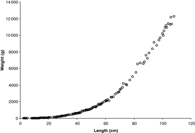
Weight–length data for cod captured in 1903 by steam trawlers from Moray Firth and Aberdeen Bay. Data lumped by 0.5 cm length class, thus one point may represent 1–12 specimens
Tyurin (1927) suggested that plotting weight–length data on double-logarithmic paper will allow fitting a straight line; Clark (1928) and Keys (1928) realized that the equation describing that line (Eqn 3) was the logarithmic equivalent of the weight–length relationship (Eqn 2). Figure 2 shows a log–log plot of Fulton's data with regression line. The logarithmic presentation not only linearizes the relationship but also corrects for the increase in variation with length visible in Fig. 1 and shows the high variation in small specimens, which at 2.5 cm length are post-larvae. If fishes smaller than 15 cm are excluded, the regression changes to: W = 0.00728L3.07 with n = 359, r2 = 0.9992, 95% CL a = 0.00703–0.00755, 95% CL b = 3.059–3.078, coefficient of variation = 0.0068. The confidence limits of a and b of this new regression do not overlap with that of the overall regression shown in the legend of Fig. 2, i.e. we can conclude that small specimens have a different WLR from larger specimens, and that the new regression better predicts weight from length within the size range for which it is likely to be used. Note also that the 95% confidence limits of b do not include 3.0, i.e. specimens ‘must increase in some other dimensions, whether breadth or thickness, in greater proportion than they increase in length’ (Fulton, 1904).
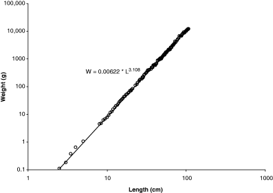
Double-logarithmic plot of data in Fig. 1. Overall regression line is W = 0.00622L3.108, with n = 468, r2 = 0.9995, 95% CL of a = 0.00608–0.00637, 95% CL of b = 3.101–3.114, and coefficient of variation = 0.0094. Note that mid-length of length classes was used, e.g. 10.25 cm for length class 10–10.49 cm and number of specimens per length class (1–12) was used as a frequency variable in the linear regression
 ()
()Thus, the predicted mean weight of a cod of 60 cm total length would be 2094 g (1891–2319 g).
Growth stanzas and inflection points
Fulton (1904) presents weight–length data for herring (Clupea harengus Linnaeus 1758), including specimens as small as 1.9 cm, i.e. the size of post-flexion larvae. As can be seen in Fig. 3, there are two growth stanzas with an inflection point at about 8 cm length, and small specimens up to 8 cm have a significantly different weight–length relationship than larger specimens. If these small specimens were included in an overall regression, b = 3.49 would be overestimated. Stergiou and Fourtouni (1991) explored growth stanzas of Zeus faber Linnaeus, 1758 and found them to be correlated with ontogenetic shifts in diet.
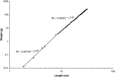
Double-logarithmic plot of Clupea harengus weight vs length based on data in Fulton (1904), showing two growth stanzas and an inflection point at about 8 cm. First growth stanza: n = 5 (92), r2 = 0.9984, 95% CL of a = 0.00125–0.00134, 95% CL of b = 3.66–3.72, and CV = −0.0219. Second growth stanza: n = 46 (400), r2 = 0.9996, 95% CL of a = 0.00301–0.00312, 95% CL of b = 3.28–3.29, CV = 0.0064
Understanding parameter b
Parameter b is the exponent of the arithmetic form of the weight–length relationship (Eqn 2), and the slope of the regression line in the logarithmic form (Eqn 3; Fig. 2). If b = 3, then small specimens in the sample under consideration have the same form and condition as large specimens. If b > 3, then large specimens have increased in height or width more than in length, either as the result of a notable ontogenetic change in body shape with size, which is rare, or because most large specimens in the sample were thicker than small specimens, which is common. Conversely, if b < 3, then large specimens have changed their body shape to become more elongated or small specimens were in better nutritional condition at the time of sampling.
Figure 4 shows the frequency distribution of mean exponent b for 1773 species. Mean b was chosen rather than including all estimates to avoid bias towards well-studied species with many estimates. The 95% confidence limits of the median did not include 3.0, i.e. there was a slight but significant tendency for most fishes to increase in thickness as they grew. Ninety percent of the values ranged from 2.7 to 3.4, thus confirming the suggestion of Carlander (1969) that the exponent b should normally fall between 2.5 and 3.5. The distribution appears about normal, although six of seven formal normality tests in Hintze (2001) rejected normality. As can be seen by comparing frequencies with the normal distribution line shown in Fig. 4, the frequencies of b values around 3.0 and below 2.3 and above 3.7 were higher than predicted by a normal distribution.
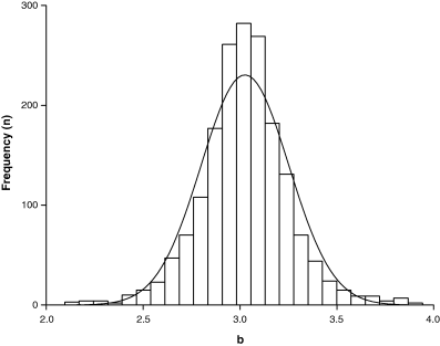
Frequency distribution of mean exponent b based on 3929 records for 1773 species, with median = 3.025, 95% CL = 3.011–3.036, 5th percentile = 2.65 and 95th percentile = 3.39, minimum = 1.96, maximum = 3.94; normal distribution line is overlaid
Carlander (1977) demonstrated that values of b < 2.5 or >3.5 are often derived from samples with narrow size ranges. Figure 5 explores the relationship between the residuals of the exponent b and the length-ranges (expressed as fractions of maximum lengths of species) that were included in estimating the respective weight–length relationships. A robust regression analysis found the slope of absolute residuals vs fraction of maximum length to be negative and significantly different from zero, i.e. residuals were becoming smaller with the increase in length-range used, thus confirming the findings of Carlander (1977).
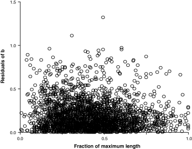
Absolute residuals of b = 3.0 plotted over length range used for establishing weight–length relationship. Length range expressed as fraction of maximum length known for the species. Robust regression analysis of absolute residuals vs fraction of maximum length resulted in n = 2,800, r2 = 0.0065, slope = −0.0505, 95% CL −0.0735 to −0.0274
Mean condition of specimens as well as the difference in condition between small and large specimens vary between seasons, localities and years, resulting in different weight–length relationships. The influence of extreme values of b on mean b decreases with the number of estimates. Figure 6 shows a plot of absolute residuals of mean b over the respective number of weight–length estimates per species. With two exceptions, all values of mean b below 2.5 or above 3.5 are based on 1–3 WLRs only, whereas – with two exceptions – all estimates of mean b that are based on five or more WLRs fall within the expected range of b = 2.5–3.5. In other words, most extreme values of mean b stem from species with only few WLRs and the mean is likely to fall into the expected range if more WLRs become available for these species. The two outliers are species with truly allometric growth, namely the red bandfish Cepola macropthalma (Linnaeus, 1758) and the blackfin icefish Chaenocephalus aceratus (Lönnberg, 1906).
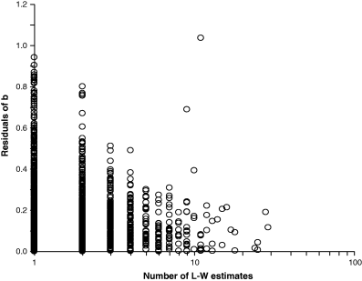
Absolute residuals of mean b per species from b = 3.0, plotted over respective number of weight–length estimates contributing to mean b, for 1773 species. Two outliers with about 10 weight–length estimates belong to species with truly allometric growth; see text
Cepola macrophthalma lives in vertical burrows from which it hunts for small crustaceans and chaetognaths (Stergiou et al., 1992; Stergiou, 1993). Apparently this life-style is favoured by an over-proportional increase in length relative to growth in weight, and this is reflected in an exponent of b ∼ 2.0 (n = 11; median = 2.05; 95% CL = 1.68–2.05).
The blackfin icefish Chaenocephalus aceratus (Lönnberg, 1906) has a planktonic elongated post-larval stage, whereas adults are less-elongated bottom-dwellers with massive heads. This change in proportions is expressed by an exponent of b ∼ 3.7 (n = 9; median = 3.67; 95% CL = 3.59–3.81).
Another example of allometric growth is the king soldierbream Argyrops spinifer (Forsskål, 1775) with b ∼ 2.5 (n = 3; median = 2.54, range = 2.46–2.65), where young fish occur in very shallow waters of sheltered bays and have a body shape similar to a butterfly fish, presumably favouring its manoeuvrability and reducing predation, whereas larger fish live in deeper waters and have a more elongated body shape, presumably favouring swimming speed (Weihs, 1973).
Note, however, that in all three examples of allometric growth it might be worthwhile to explore the existence of growth stanzas, e.g. by examining the linearity of plots of log W vs log L, and calculating separate weight–length relationships for these stanzas, which may have less extreme values of b.
In summary, when discussing the exponent b of single weight–length relationships one should refer to differences in condition between small and large individuals in the respective area at that point in time. Only when all available weight–length estimates are considered and are likely to reasonably cover geographic, seasonal, and inter-annual variation does it make sense to discuss isometric versus allometric growth of the species as a whole, based on mean b. Strong allometric growth patterns are rare and should be accompanied by an examination of growth stanzas and a discussion of the potential evolutionary benefits associated with such ontogenetic change in body proportions.
Understanding parameter a
Parameter a is the coefficient of the arithmetic weight–length relationship (Eqn 2) and the intercept of the logarithmic form (Eqn 3). Figure 7 shows the frequency distribution of mean log a for 1773 species. Mean log a per species was chosen rather than including all estimates to avoid bias towards well-studied species with many estimates. Ninety percent of the values ranged between 0.001 and 0.05. The distribution is roughly log-normal but strongly skewed to the left, i.e. there were more species with small values of a than predicted by a log-normal distribution.
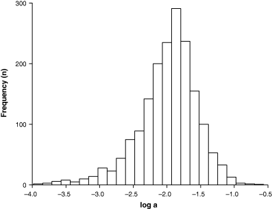
Frequency distribution of mean log a based on 3929 records for 1773 species, with median a = 0.01184, 95% CL = 0.0111–0.0123, 5th percentile = 0.00143, 95th percentile = 0.0451, minimum = 0.0001, and maximum = 0.273
From the logarithmic form of the weight–length relationship (Eqn 3) and from the corresponding plot of weight versus length (Fig. 2) it is evident that every decrease in the slope of the regression line will lead to an increase in the intercept, and vice-versa. Froese (2000) points out that if several weight–length relationships are available for a species, then a plot of log a over b will form a straight line and can be used to detect outliers. For example, 25 estimates of weight–length relationships were available for the gila trout, Oncorhynchus gilae (Miller, 1950), from various streams in the Gila River system in New Mexico (Probst and Stefferud, 1997). Parameter a is log-normally distributed with geometric mean a = 0.0099, 95% confidence limits of 0.0072–0.0137, and total range of values from 0.002 to 0.086. Exponent b is normally distributed with mean b = 3.012, 95% confidence limits of 2.948–3.075, and total range of values from 2.60 to 3.32. The 95% confidence limits of the mean include 3.0 and thus the overall growth pattern of the species is isometric. A robust regression analysis of log a over b identifies one outlier and after its removal linear regression explains 99% of the remaining variance (Fig. 8). In other words, the strong interrelationship between parameters a and b is linearized in a plot of log a over b and helps in detecting WLRs that are questionable because of e.g. narrow size range, few data with high variance, or outliers in the respective sample. In some cases, outliers could be a misidentification of a similar-looking species, or a population that differs in body shape from the others.
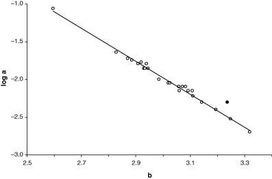
Plot of log a over b for 25 weight–length relationships of Oncorhynchus gilae. Black dot identified as outlier (see text) by robust regression analysis (robust weight = 0.000). Regression line: log a = 4.544–2.174b, n = 24, r2 = 0.9902, CV = −0.0167
Froese (2000) and Kulbicki et al. (2005) show multi-species plots of log a over b to demonstrate the interdependence of these parameters. Here I repeated this plot (Fig. 9) using the means of the parameters per species to avoid bias towards well-studied species with many estimates, and to reduce the effect of intra-specific variability referred to above. Also, similar to Kulbicki et al. (2005), I used different symbols for different body shapes obtained from fishbase. A dotted line at b = 3.0 was inserted to indicate the areas of negative-allometric, isometric and positive-allometric growth. Note that, as discussed above in the context of Fig. 6, many points below b = 2.5 and above b = 3.5 are based on only very few WLRs and are likely to move closer to the centre of the graph when more estimates become available for these species.
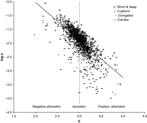
Scatter plot of mean log a (TL) over mean b for 1223 fish species with body shape information (see legend). Areas of negative allometric, isometric and positive allometric change in body weight relative to body length are indicated. Regression line based on robust regression analysis for fusiform species, with n = 451, intercept = 2.322–0.133 = 2.189, and slope as in Eqn 17
As can be seen from the distribution of the different symbols relative to the regression line in Fig. 9, the variation in log a is largely a function of the body shape of the respective species. A robust multiple regression of log a as a function of b and body shape as a categorical variable explains 82% of the variance in Fig. 9 and results in:
 ()
()One can interpret Eqn 17 as having the same slope as the regression line shown in Fig. 9 but being moved up or down along the dotted line, depending on the body shape of the fishes under consideration. Thus, most of the considerable variance in Fig. 9 can be accounted for by differences in body shape, allometric vs isometric growth patterns, and insufficient data for reliable estimation of mean values for a and b for some species.
Form factor
 ()
()If not enough WLRs are available for the species or population in question for estimating the regression of log a vs b, then the mean slope S = −1.358 from Eqn 17 can be used as proxy for estimating the form factor.
The form factor a3.0 can be used to determine whether the body shape of a given population or species is significantly different from others. For example, fishbase 12/2005 contained nine weight–length relationships for Gadus morhua from the North Sea and four from the Baltic. If we had a hypothesis that body shape of cod in the Baltic were different from the North Sea, we would calculate the respective form factors from Eqn 18 and perform a two-sample t-test on log a3.0. This results in the null-hypothesis being accepted [t-value = 0.6263, prob. level = 0.5439, power (0.05) = 0.08844], i.e. there is no significant difference in body shape between these populations.
In Fig. 10 the relationship of the form factor with body shapes of fishes is explored. There is a clear and significant increase of median a3.0 from eel-like to elongated, fusiform and short or deep body shapes (Table 1). This confirms the interpretation of a3.0 as a form factor and as an indicator of the body shape of fishes, but note the overlap of ranges, which does not allow assigning body shape based only on the form factor.
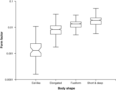
| Body shape | Median a3.0 | 95% CL | 5th–95th Percentile | n |
|---|---|---|---|---|
| Eel-like | 0.00131 | 0.00099–0.00165 | 0.00032–0.0139 | 45 |
| Elongated | 0.00838 | 0.00775–0.00906 | 0.00293–0.0178 | 403 |
| Fusiform | 0.0137 | 0.0131–0.0140 | 0.0061–0.0240 | 451 |
| Short and deep | 0.0187 | 0.0172–0.0193 | 0.0077–0.0336 | 324 |
As pointed out by Kulbicki et al. (2005), there seem to be viability limits as to how elongated or spherical a fish can be. From the 5th percentile of eel-like fishes in Table 1 we can derive a lower ‘thinness’ limit of the form factor a3.0 of 0.00032, which is about 0.03% of the volume given by the cube of body length. Similarly, from the 95th percentile of short and deep fishes in Table 1 we can derive an upper ‘plumpness’ limit of the form factor a3.0 of 0.0361, which is about 4% of the length cubed. The latter appears low and would increase if we had considered standard length instead of total length, i.e. excluding the length of the caudal fin from calculating the cube of length.
Kulbicki et al. (2005) analysed body proportions and weight–length relationships for 396 species of fishes from New Caledonia. They provided guidance for estimating preliminary WLRs for fishes where none were available, based on seven measurements that could be taken from suitable pictures, plus a classification as to whether the species is flat or laterally compressed, oval, or round in cross-section. Here I provide a simplified version of that approach, i.e. a very preliminary WLR for a species where none exists can be derived by using the median value of parameter a3.0 based on the respective body shape of the species from Table 1, and setting exponent b to 3.0. A better preliminary estimate can be obtained if at least one specimen within the size-range of interest is available, length and weight are measured, exponent b is set to 3.0, and the coefficient a is obtained from a = W/L3.
Condition factor
Heincke (1908) established the usefulness of Fulton's condition factor (Eqn 1) for comparing seasonal changes in nutritional condition. This is best done by a double-logarithmic plot of condition over length, where the connected points will form a more or less straight line. Alternatively, respective WLRs can be transformed to condition at length using Eqn 4. For example, the comber Serranus cabrilla (Linnaeus, 1758) in the Aegean Sea has seasonal WLRs with spring a = 0.0326, b = 2.601; summer a = 0.0207, b = 2.767; autumn a = 0.0126, b = 2.955; and winter a = 0.0135, b = 2.914 (Moutopoulos and Stergiou, 2002). In all seasons reported here, large specimens have lower condition than small specimens, as indicated by exponent b < 3 and shown in Fig. 11. This trend is least expressed in autumn and winter, when small and large specimens have about the same condition, and is most expressed in spring during the spawning season. The dotted line is based on geometric mean a and mean b (see below) of all WLRs of this species, including other areas. It shows that the Aegean Sea population, except for small specimens in spring and large specimens in autumn and winter, has a lower condition than the average for this species.
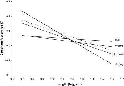
Log–log plot of condition vs length calculated from weight–length relationships of Serranus cabrilla taken in spring, summer, autumn and winter in the Aegean Sea, respectively. Dotted line shows condition factors associated with geometric mean a and mean b across all available WLRs for this species
 ()
() ()
() ()
()For most iteroparous fishes Lopt falls between the first and second spawning, thus making overfishing theoretically impossible, because all fish had a chance to spawn before being caught (Myers and Mertz, 1998). But as Heincke (1908) already pointed out, a further increase of e.g. 16% in mussel weight per specimen of North Sea plaice can be obtained if fish are caught when condition is highest in the non-spawning season. For example, if we assume a maximum total length of the comber in the Aegean Sea of 28 cm, we obtain from Eqn 21 an asymptotic length of 29.4 cm and from Eqn 20 the length at optimum size as 18.0 cm, which is about the same as the size of females at first maturity (Papaconstantinou et al., 1994). Using Eqn 4 with optimum length and the seasonal WLRs presented above, we obtain the following mean condition factors: spring K = 1.03, summer K = 1.06, autumn K = 1.11, and winter K = 1.05. Spawning season for this species is in spring and summer. Catching comber in the Aegean Sea only around 18 cm total length in autumn would thus deliver specimens in best condition (5–8% more weight per specimen than in other seasons), with least impact on the stock.
Relative condition and relative weight
 ()
()For example, if we revisit the seasonal condition estimates for Serranus cabrilla in the Aegean Sea (Fig. 11), we can now express these as relative weights of a medium-size fish of 20 cm total length and find that these were 89.3% in spring, 93.2% in summer, 99.7% in autumn and 94.5% in winter. Medium size specimens in this Aegean Sea population apparently do not reach and surpass 100% of mean weight, confirming a hypothesis by Stergiou et al. (1997) that fishes in the oligotroph eastern Mediterranean have lower weight at length than those in the central and western Mediterranean.
Recommendations
Within-species variance in weight–length relationships can be substantial, depending on the season, the population, or annual differences in environmental conditions. As a result, differences in weight estimated from length can be two-fold or more, depending on which relationship is chosen. Thus, if at all possible, one may want to re-estimate weight–length relationships for the specimens under study. The following guidelines for data collection and analysis of weight–length relationships can be given:
- 1
Make certain that the gear used for collecting specimens do not introduce a bias with respect to length or weight, such as can be the case if only one size of gill net is used; gill nets tend to select fat fish among the shorter ones and thin fish among the longer ones, thus introducing a bias in b (Kipling, 1962).
- 2
When selecting specimens for measuring weight–length data, strive to include the size range to which the relationship will later be applied. Do not include early juveniles, such as fry and fingerlings, which in most fishes have not yet obtained adult body shape (Le Cren, 1951; Carlander, 1969; Murphy et al., 1990; Safran, 1992). If needed, estimate separate length–weight relationships for different development phases or growth stanzas (see Fig. 3). Also, do not include very old specimens, which often have distorted body forms with unusually high proportions of fat. Obviously aberrant specimens that are unusually thin or that are stunted or otherwise distorted should not be included.
- 3
Strive to include about equal numbers of randomly selected small, medium-size and large specimens. There is no need to measure large numbers of abundant medium-size specimens, as these have little influence on the relationship. For example, 10 small, 10 medium-size and 10 large specimens will normally suffice to establish a reliable length–weight relationship. If specimens are rare, lower numbers will also be acceptable.
- 4
If only one or few specimens of similar size are available, set b = 3 and determine a from a = W/L3; take the geometric mean of a in case of several specimens.
- 5
When planning data collection, try to sample as many months as possible. Analyse samples by month to detect seasonal variation.
- 6
Test for differences between sexes. If such differences are significant, present separate relationships for males, females, and both sexes.
- 7
When selecting published weight–length relationships for use elsewhere, choose a relationship where data were sampled in the same season in the same or adjacent areas. If such studies are not available, take a study with parameters close to the median of a and b over all available studies. Alternatively, use geometric mean a and mean b across all available studies.
- 8
When discussing within-species variation in weight–length relationships, first do a log a vs b plot to detect and exclude outliers. Then focus on variation in condition, which is likely to be driving variation in parameters a and b, e.g. with the help of a log K vs log L plot (Fig. 11). Try to find and explain e.g. seasonal, geographic, climatic or other patterns in the variation of the condition factor.
- 9
When exploring relative condition of individuals within a sample, use Le Cren's (1951) relative condition factor (Eqn 5). When exploring relative condition across populations or species, use relative weight in relation to mean weight (Eqn 22).
- 10
When exploring isometric vs allometric growth, use mean b and discuss whether the available length–weight studies cover a wide-enough seasonal and geographical range to be representative for the species. If strong allometric growth is found, try to find the reasons for such significant changes in body proportions.
- 11
When discussing across-species variation in length–weight relationships, use mean values of b and log a by species. You would expect the overall mean of b to be close to 3.0, but there may be, for example, phylogenetic or functional groups of fishes with a tendency for allometric growth. You may want to calculate and discuss the general form factor (Eqn 18), which is likely to differ between phylogenetic or functional groups of fishes, or between riverine or lacustrine habitats.
- 12
When presenting weight–length relationships, make sure to indicate the number of specimens processed, range and type of length measurements, units (preferably grams and centimetres, to reduce the number of digits in a and facilitate comparisons between studies), parameters a and b with their respective 95% confidence limits, and the coefficient of correlation. Make your WLRs available to fishbase (http://www.fishbase.org), so that they can be archived and used by others.
Acknowledgements
I thank Crispina Binohlan for compiling and standardizing most of the weight–length relationships used in this study. I thank Crispina Binohlan, Daniel Pauly, Kostas Stergiou and Amanda Stern-Pirlot for useful comments on the manuscript. I thank Barbara Schmidt and the staff of the IFM-GEOMAR library for their fast and competent help with tracing old publications. This publication was supported in part by the EC project INCOFISH (INCO-CT-2005-003739).


