Effective measures to counter the rising levels of carbon dioxide in the Earth's atmosphere require that we better understand the functioning of the global carbon cycle. Uncertainties about, in particular, the terrestrial carbon cycle's response to climate change remain high. We use a well-known stochastic inversion technique originally developed in nuclear physics, the Metropolis algorithm, to determine the full probability density functions (PDFs) of parameters of a terrestrial ecosystem model. By thus assimilating half-hourly eddy covariance measurements of CO₂ and water fluxes, we can substantially reduce the uncertainty of approximately five model parameters, depending on prior uncertainties. Further analysis of the posterior PDF shows that almost all parameters are nearly Gaussian distributed, and reveals some distinct groups of parameters that are constrained together. We show that after assimilating only 7 days of measurements, uncertainties for net carbon uptake over 2 years for the forest site can be substantially reduced, with the median estimate in excellent agreement with measurements.

Introduction

Only about half of the increasing emissions of CO₂ from human activities currently remain in the atmosphere (Prentice et al., 2001). The remainder is taken up by both the oceans and the terrestrial biosphere, to roughly equal amounts (Joos et al., 2003). This current carbon sink in the terrestrial biosphere is, by some models at least, predicted to turn into a source (Cox et al., 2000; Cramer et al., 2001; Friedlingstein et al., 2003). Better quantification of the exchange fluxes of CO₂ between the terrestrial biosphere and the atmosphere and better understanding of the underlying processes are therefore of foremost importance for the design of efficient climate protection strategies. Terrestrial ecosystem models (TEMs) have been used extensively to study the processes leading to either carbon loss or gain by the land biota (McGuire et al., 2001; Prentice et al., 2001). However, results still vary significantly because of differences between models (Cramer et al., 1999). While only very few studies using TEMs have considered uncertainties in fluxes as a result of parameter uncertainties, Knorr & Heimann (2001a, b) have shown that uncertainties of TEM process parameters lead at least to the same spread of simulated atmosphere–vegetation carbon fluxes as intermodel differences.

More recently, Kaminski et al. (2002) have shown that TEMs can be combined with atmospheric transport inversion techniques. By using an additional process model and a Bayesian approach to parameter inversion, such inversions are both better constrained than transport inversions and allow inferences about the underlying processes. An example of a more complex Carbon Cycle Data Assimilation System (CCDAS) is given by Rayner et al. (2005). CCDAS requires one to specify prior means and error covariance matrices of model parameters, as an approximation of the prior probability density function (PDF) of parameters. To generate and analyze such a PDF is one purpose of the present study.

Few attempts exist at quantifying uncertainty ranges based directly on experimental data (Knorr, 2000; White et al., 2000; Knorr & Heimann, 2001a). It is, therefore, of general interest to utilize the still growing amount of eddy covariance measurements of CO₂ and water fluxes (FLUXNET, Global Carbon Project, 2003) for ecosystem model parameter estimation. Wang et al. (2001) used a non-Bayesian parameter optimization and showed that for their model, up to five parameters could be estimated on the basis of eddy covariance measurements of CO₂, water, heat and ground heat fluxes. Prior knowledge of parameter values was used to initialize the parameters that were optimized, to set the parameters that remained unaffected by the optimization, and to determine reasonable limits for the space of parameter solutions allowed. The result is a set of model parameters that are either based fully on prior estimates, or fully on the inversion against measurements.

Here, Bayesian methods offer a more consistent approach by combining prior knowledge with the additional information gained from the inversion. This does not only allow the simultaneous determination of all parameters, it also allows considering prior knowledge consistently for all parameters. Weakly constrained parameters are, therefore, given an appropriate uncertainty range instead of being excluded a priori from the optimization. The method can be applied to global scale inversions (Rayner et al., 2005), or to sites using flux measurements as a model constraint.

With this contribution, we will demonstrate a general method for Bayesian parameter estimation of complex, process-based TEM, where parameter uncertainty ranges are derived from systematic sampling of the complete PDF. By comparing prior and posterior uncertainty ranges of parameters, it will be determined which parameters can be constrained by eddy covariance measurements of CO₂ and water fluxes for a given set of prior parameter uncertainties and for a given measurement error, using a particular TEM. The analysis of covariances is then used to determine which parameter values cannot be determined independently by the data. Finally, simulations with the constrained model – using both the complete PDF or its first two moments – are carried out for much longer time series than those used during the parameter estimation, to test the validity of the parameterization across time. Here, we also assess whether an approximation to the full PDF as used by CCDAS (means and error covariances) sufficiently represents uncertainties in net CO₂ fluxes. The method is thus presented as a prototype for an initial step of CCDAS that allows the exploitation of widely available site-specific flux data through constraining model parameters.

Methods

Monte Carlo inversion

The given task of this study is to determine the probability distribution of a vector of model parameters p, given a set of measurements f, in this case fluxes. Whether a given vector p agrees with f is determined by running the model M, such that

(1)

f_M is the vector of model-simulated measurements, and c and s vectors of environmental boundary conditions and model state variables, respectively. f, f_M, c and s contain values across both time and types of data (CO₂, water and heat fluxes; temperature, solar radiation, humidity; soil moisture and leaf area index (LAI)), while p is assumed invariable in time. For a process-based TEM, M is usually nonlinear and too complex to be expressed as a set of standard mathematical functions. According to Mosegaard (1998), this amounts to a general inverse problem that can most efficiently be solved by direct sampling of the PDF in parameter space using Monte Carlo techniques. Developed for applications in nuclear physics (Metropolis et al., 1953), and later geophysics (Mosegaard & Tarantola, 1995; Mosegaard, 1998; Mosegaard & Rygaard-Hjalsted, 1999), it is now widely used in other fields of environmental modeling. It consists of a stochastic technique that generates a random set of points p¹, …, p^N in parameter space with a distribution that approximates any given function f(p) for large values of N. For a Bayesian inversion, this function is chosen as the posterior PDF of model parameters, given by

(2)

with a normalization constant, ν (Mosegaard & Sambridge, 2002). L(p) is the likelihood function, which expresses the misfit between model-derived values and measurements in relation to measurement error, and ρ(p) is the prior probability distribution of parameters. Errors representing missing or incorrect processes were neglected in this study. The likelihood function is expressed as the negative exponential of the misfit against measurements, J_f(p), such that

((3a))

with

((3b))

C_f is the error covariance matrix of the measurements, and the superscript T denotes the transposed vector. Similarly, the prior probability, ρ(p), can be written as

((4a))

and

((4b))

with p₀, the vector of prior parameter values, and C_p, the error covariance matrix of the priors. The formulation assumes Gaussian uncertainties for both prior parameters, p, and the assimilated data, f.

Standard inversion techniques aim at inferring the global minimum of the function, J(p)=exp{–f(p)}. In the case of Monte Carlo inversion, the generated series of sample points, p¹, …, p^N, simply has a distribution with its highest density in the vicinity of the maximum of f(p). If the objective is to gain understanding of the probability distribution of parameters rather than to find the exact optimum, this technique has obvious advantages. The sampled distribution can subsequently be used to compute the expected value of any desired variable or expression, x, under the predefined PDF, f(p):

(5)

To assess to what degree the distribution of model parameters deviates from a Gaussian one, it is also possible to compute the projection of the multidimensional PDF onto the dimension of a single parameter (importance sampling) from

(6)

I_a,b(x) denotes the interval function, which is 1 if a≤x<b, else 0, and ɛ an appropriately chosen resolution parameter.

The complete method of Monte Carlo inversion is described in detail by Mosegaard & Tarantola (1995) and reviewed by Mosegaard & Sambridge (2002). We always perform one iteration starting from the prior set of parameters (i.e. p¹=p₀). For some cases (see Results), we add an ensemble of Monte Carlo integrations with varying starting points in the way suggested by Gelman et al. (1995). To generate subsequent values p², p³, … in each series, a new point is tried by varying all vector elements by some step, Δp, chosen with a Gaussian distributed random number generator with mean zero and standard deviation set for each parameter separately to the prior uncertainty times an appropriately chosen step-length factor. The new point, pⁱ+Δp at step i of the iteration, is accepted or rejected according to a two-step version of the Metropolis algorithm: The first step is always accepted, if ρ(pⁱ+Δp)/ρ(p)≥1, and it is accepted with a probability of ρ(pⁱ+Δp)/ρ(p) if ρ(pⁱ+Δp)/ρ(p)<1. Acceptance with a probability of <1 – the latter case – is carried out by generating a uniformly distributed random number between 0 and 1. Only if this number is less than the chosen probability, the first step is accepted. The second step is assessed in the same way as the first, except that the prior probability ρ(p) is replaced by the likelihood function L(p). Only if both steps are accepted, the next point in the series is pⁱ⁺¹=pⁱ+Δp, else pⁱ⁺¹=pⁱ (i.e. the previous point is chosen again). We adjust the step length for each parameter to values which lead to an average acceptance rate of the new points around 0.3 (Gelman et al., 1995). Only the second step requires model execution.

Simulations

As a demonstration of the Monte Carlo method, we chose two different photosynthesis models and two setups with a reduced and a more extensive part of the Biosphere Energy-Transfer Hydrology (BETHY) model. The reduced version of BETHY is used together with the C4 photosynthesis model and excludes the heterotrophic respiration part. Compared with the C3 version with heterotrophic respiration, this reduces the number of free parameters from 23 to 14. The C4 version uses eddy covariance measurements, by Kim & Verma (1991), from the first ISLSCP field experiment (FIFE) grassland experimental site in Kansas, and the C3 version data from the Loobos pine forest site in the Netherlands (Dolman et al., 2002).

Input and flux data

The FIFE site in north-eastern Kansas, USA (39°03′N, 96°32′W) was dominated by the C4 tallgrass species Andropogon gerardii, Sorghastrum nutans and Panicum virgatum. The implementation of BETHY for this site is also described by Knorr (1997). In this case, we assimilated daytime data of net canopy assimilation (gross primary productivity (GPP) minus total-canopy leaf respiration) derived from eddy covariance measurements of net ecosystem exchange (NEE) by subtracting soil and plant, excluding leaf, respiration rates derived from night-time CO₂ fluxes, for 4 days representative of the 1987 growing season: June 5, July 2, July 30, and August 20. July 30 was the only date with severe drought. We also assimilated daytime canopy conductance values for the same dates and times that were obtained through inversion of the Penman–Monteith equation against daytime latent energy flux measurements. Photosynthetically active radiation (PAR), air temperature, vapor pressure deficit (VPD) and relative plant available soil moisture (w/w_m, Eqns (A12) and (A17)) were used as input data. All data were taken from Kim & Verma (1991). Global radiation was computed from Julian day, longitude and latitude, while wind speed and free-air CO₂ concentration were left constant at 3 m s⁻¹ and 355 ppm, respectively. We used a relative uncertainty of 20% for both net canopy assimilation and canopy conductance, with a threshold of 3.0 μmol m⁻² s⁻¹ and 1.5 mm s⁻¹, respectively.

The vegetation at the Loobos site (the Netherlands, 52°10′N, 5°74′E) was dominated by Pinus sylvestris with an understory of the grass Deschampsia flexuosa (Dolman et al., 2002). Global radiation, PAR, air temperature, ambient CO₂ concentration, wind speed, VPD and total soil water content, w_tot, were used as input data. Soil water content at wilting point (2.5% vol.) and at field capacity (12.4% vol.) were estimated from soil texture information. We assimilated half hourly values of NEE and latent energy flux (LE) from 7 days, 5 in 1997 (January 14, March 3, July 9, September 24, October 25), and 2 in 1998 (May 15, August 9). Those days were chosen to represent typical conditions of the various seasons, have as complete data coverage as possible, and at least some cloud-free conditions during daytime. We also required that there was no rainfall during the day and the day before so that soil and canopy evaporation could be neglected. The uncertainty of NEE was taken to be 20% of NEE during day and 50% of NEE during night, accounting for low wind speed and little turbulence during night-times. The minimum uncertainty threshold was set to 3.0 μmol m⁻² s⁻¹. Uncertainties of LE were considered to be 20% of LE, with a threshold of 22.0 W m⁻². Uncertainties of input data were not considered for either site.

Prior model parameter values and uncertainties

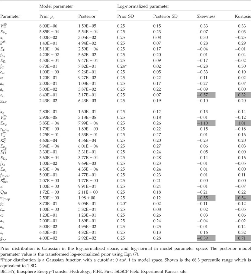
All model parameters and their prior values are listed in Table 1. Their choice is based on the model description of BETHY (Knorr, 2000), with a few exceptions: the value for r_JmV_m was derived from data by Wullschleger (1993), Medlyn et al. (2002) and Leuning (2002); k²⁵ and E_k follow Knorr (1997); E_Rd was set to the value cited by Kim & Verma (1991); f_R,leaf was modified for one plant respiration rate instead of separate maintenance and growth respiration; R_het⁰ was set to a value for which the heterotrophic respiration model (at a priori parameter values) driven with data from the Loobos site reproduces the range of measured soil respiration rates given in Raich et al. (2002) and Reichstein et al. (2003); Q₁₀ follows Raich et al. (2002); w_pwp was derived from soil texture information and soil water potential relations from Schachtschabel et al. (1992); and a_v was set to the upper bound of values given by Knorr (2000).

Table 1. Parameters of BETHY that were used as priors in the inversion against eddy covariance measurements

Symbol	Description	Value	Unit	Eqn	C3	C4
Photosynthesis
α_q	Quantum efficiency of photon capture (C3)	0.28	mol(e⁻) mol⁻¹	A1c	X
V_m²⁵	Maximum carboxylation rate at 25°C (C3)	29	μmol m⁻² s⁻¹	A2	X
V_m²⁵	Maximum carboxylation rate at 25°C (C4)	8	μmol m⁻² s⁻¹	A2		X
E_Vm	Activation energy of V_m	58 520	J mol⁻¹	A2	X	X
r_JmV_m	Ratio of J_m to V_m at 25°C	1.79	–	A3	X
Γ_*²⁵	CO₂ compensation point without dark respiration at 25°C	42.5	μmol mol⁻¹	A4	X
K_C²⁵	Michaelis–Menten constant for carboxylation at 25°C	460	μmol mol⁻¹	A5	X
E_KC	Activation energy of K_C	59 356	J mol⁻¹	A5	X
K_O²⁵	Michaelis–Menten constant for carboxylation at 25°C	0.33	mol mol⁻¹	A6	X
E_KO	Activation energy of K_O	35 948	J mol⁻¹	A6	X
α_i	Quantum efficiency of photon capture (C4)	0.04	mol(CO₂) mol⁻¹	A7		X
k²⁵	CO₂ specificity at 25°C	0.14	mol m⁻² s⁻¹	A8		X
E_k	Activation energy of k	50 967	J mol⁻¹	A8		X
Carbon balance
f_Rd	Ratio of leaf dark respiration at 25°C and V_m²⁵ (C3)	0.011	–	A10	X
f_Rd	Ratio of leaf dark respiration at 25°C and V_m²⁵ (C4)	0.042	–	A10		X
E_Rd	Activation energy of leaf dark respiration	45 000	J mol⁻¹	A10	X	X
f_R,leaf	Ratio of canopy to total plant respiration	0.5	–	A11	X
R _het ⁰	Heterotrophic respiration at 0°C and field capacity	2.07	μmol m⁻² s⁻¹	A12	X
κ	Soil moisture factor of heterotrophic respiration	1	–	A12	X
Q₁₀	Temperature dependency of heterotrophic respiration	1.72	–	A12	X
Stomatal control
w_pwp	Soil water content at permanent wilting point	2.5	vol%	–	X
f_Ci	Non water limited ratio of C_i,0 and C_a (C)	0.87	–	A14	X
f_Ci	Non water limited ratio of C_i,0 and C_a (C4)	0.67	–	A14		X
c_w	Maximum water supply rate of root system	1	mm h⁻¹	A17	X	X
Energy and radiation balance
ω	Single scattering albedo of leaves	0.12	–	–	X	X
a_v	Albedo of close vegetation surface cover	0.2	–	A18	X	X
a_s	Fraction of solar radiation absorbed by soil under close canopy	0.05	–	A18	X	X
ɛ_s	Sky emissivity factor	0.64	–	A19	X	X
g_a,v	Vegetation factor of atmospheric conductance	0.04	–	A20	X

BETHY, Biosphere Energy-Transfer Hydrology.

We distinguish between model parameters (Table 1) and parameters used by the Metropolis algorithm written p={p₁, …, p_N}. For the model parameters, we assume a priori that (a) they are always greater than zero and (b) that they have a log-normal distribution. The parameters used by the optimization will be called log-normal parameters and have a prior value of 1 and a prior uncertainty of 0.125, 0.25, and 0.5. The log-normalized parameters have a prior distribution that is Gaussian (Eqn (4b)). To transform from log-normalized parameter, p, to model parameter p_i (see previous section), we use the following equation:

(7)

p_i,0 is the prior value in model parameter space as listed in Table 1. Note that throughout the remainder of this analysis, we will show and discuss exclusively the log-normalized parameters (with the exception of Table 3), because their prior values are identical (1.0) and their posterior values easier to intercompare.

Table 3. Prior and posterior parameter values in model space for FIFE (above, BETHY C4 version), and Loobos (below, BETHY C3 version); prior parameter and standard deviation (SD) in log-normalized space; posterior parameter with SD, skewness and kurtosis, also in normalized space (strongly non-Gaussian parameters highlighted)

An exceptional model parameter is f_Ci, for which we require 0≤f_C≤1. Instead of a log-normal distribution in model parameter space, we choose a probability distribution that is defined by a normal distribution but is cut off at 0 and 1. f_Ci,0 is the prior estimate of f_Ci, and f_Ci=p_kf_Ci,0 replaces Eqn (7), where k is the parameter index for f_Ci.

The vector of prior log-normalized parameters is thus p₀={1, …, 1}, and C_p, the error covariance matrix of the priors:

where x is 0.125, 0.25, or 0.5, as above. Covariances for priors are assumed to be zero. For the prior probability distribution, ρ(p) (Eqns (4)), we have the additional condition

Results

We will, first, show results to demonstrate convergence of the algorithm. Next, optimized parameter values will be described by their means, standard errors, and covariances, all in the space of log-normalized parameters (cf. Eqn (7)). Comparison with prior means and errors indicates about how many parameters we have learned something through the assimilation of the eddy covariance data. We also assess for which parameters the posterior PDF differs from the Gaussian distribution assumed for the prior PDF. For the Loobos site, we eventually compute the cumulative NEE with and without optimized parameters over a period of 2 years to test the validity of parameterizations across time and to assess to what degree the inversion has lead to a constraint on the modeled longer-term ecosystem carbon balance.

Convergence of the algorithm

To insure convergence, we performed rather long integrations with 500 000 iterations (and more in one case). For the two cases with 0.25 prior uncertainty, we produced a series of six independent simulations starting from different points in parameter space: the prior parameter vector, p₀={1, …, 1} in the space of log-normalized parameters, and points shifted away from the estimated posterior optimum, p′, by one to several times the posterior standard deviations, σ′={σ′₁, …, σ′_n} estimated from preliminary simulations. For FIFE, the starting points were p₀, p′+σ′, p′+2σ′, p′+3σ′, p′−σ′, p′−2σ′, for Loobos p₀, p′+2σ′, p′−2σ′, p′+4σ′, p′+4{+σ′₁, −σ′₂, +σ′₃, …} and p′−4{+σ′₁, −σ′₂, +σ′₃, …}. Sampling was done at every 10th iteration to avoid correlations between subsequent samplings (i.e. 500 000 iterations yielded 50 000 samplings of parameters of interest sampled according to Eqn (5)). To determine at which iteration the sequences have converged to a common maximum, as opposed to sampling around local maxima, we applied Gelman's criterion of convergence (Gelman et al., 1995) for all parameters. This test of convergence, designed for practical purposes, yields a reduction factor defined as the square root of the ratio of the mean variances of the various sequences divided by the variance of the means yielded by each sequence. This reduction factor is sampled from exactly the second half of the series up to the iteration indicated (see below the discussion of ‘burn-in time’, and Fig. 1e, f). If all sequences sample the same area of the parameter space, the reduction factor will approach a value of one, values much greater than one indicate sampling of different regions around local minima by the different sequences.

Details are in the caption following the image — **Figure 1**
Open in figure viewer PowerPoint

Convergence of the Monte Carlo inversion for 0.25 prior uncertainty of the log-normalized parameters, for the FIFE (left: a, c, e), and the Loobos site (right: b, d, f). (a, b) Estimated mean of selected parameters depending on number of iterations; (c, d) phase diagram of the two contributions to the total cost function, measuring deviation from prior parameters and between measured and modeled diagnostics (=fluxes), for sequences with varying starting points; (e, f) Gelman's reduction factor for the same parameters as above, and for two parameter products. The selected parameters are: the slowest converging, one fast converging, and the one most highly correlated with the first.

The parameters that took longest to reach a common maximum, according to Gelman's criterion, were α_i for FIFE and f_Ci for Loobos. The evolution of the estimated mean values is shown in Fig. 1a and b, respectively, again for every 10th iteration. Also shown are one fast converging parameter, and the parameter that was most highly correlated to the first. Note that in Fig. 1b, E_Vm appears to be converging more slowly than f_Ci. The explanation is that E_Vm remains highly uncertain and, as we will see later, assumes an extremely non-Gaussian distribution within the posterior PDF. In general, parameters for the FIFE site seem to converge faster than for Loobos, which would be expected for an inversion with 14 instead of 23 parameters.

A more convenient way to visualize convergence of the sampling sequences is a phase diagram using the costs of the prior probability (Eqn (4b), costs of parameters) and the misfit in the Likelihood function (Eqn (3b), costs of diagnostics) as the two axes (Gelman et al., 1995). As Fig. 1c and d shows for both sites and 0.25 prior uncertainty, all sequences appear to converge against a common global cost function minimum (maximum of the PDF), despite widely varying starting points. The convergence, however, is less straight for FIFE, where a local minimum with a cost of diagnostics of around 500 is initially reached by some of the simulations. Analysis of the other simulations (not shown) reveals that the sequence with 0.125 prior uncertainties remains even longer in a similar local minimum until it reaches a region with costs of diagnostics and parameters both around 200. The simulation with 0.5 prior uncertainty does not seem to find a local minimum and converges more rapidly, with costs of diagnostics around 100, and costs of parameters around 35.

The ratio of the costs of diagnostics over parameters in the region of the global minimum gives an indication of how strongly the inversions are constrained by observations. For the FIFE site, this ratio varies between around 1, 2, and 3 for 0.125, 0.25, and 0.5 prior uncertainties. For Loobos, the costs of diagnostics decrease only about 10% from 0.125 to 0.5 prior uncertainties, and the costs of parameters all lie around 40, giving an almost constant ratio of around 10. Apparently, the more reduced model version with 14 parameters needs rather weak constraints on parameters to converge efficiently, and is still less constrained by observations than the more direct inversion against NEE and LE. Note, however, that the FIFE inversion used only 4 days and only data from daytime fluxes.

To determine a practical initial cut-off for iterations before convergence to the global PDF maximum, the so-called ‘burn-in time’ with length n iterations, we used again Gelman's test (Gelman & Rubin, 1992; Cowles & Carlin, 1996). It requires that the reduction factor computed for the ensuing n iterations (i.e. iterations n+1 to 2n) reaches a value of around 1.2–1.4 for all sampled quantities of interest. Figure 1e and f show this reduction factor for the same parameters as Fig. 1a and b, together with the values of the product of the slowest converging parameter with the two others, as a function of the total number of simulations, variable burn-in time plus ensuing iterations of the same length. Products are required to compute parameter covariances and appear to converge at least as rapidly as the slowest parameter. (The reduction factor is always applied to the second half of the iterations up to the number indicated. A burn-in time of n=50 000 thus corresponds to 100 000 iterations.) To be on the safe side, we chose a burn-in time of length n=50 000 iterations.

Convergence of parameters for the cases with 0.125 and 0.5 prior uncertainties was evaluated by plotting expected values of all parameters against the length of the burn-in time. The same burn-in time of 50 000 iterations was found to be sufficient for all cases except for FIFE with 0.125 prior uncertainty, where 1 000 000 iterations were chosen instead. For the case of 0.25 prior uncertainty, we carried out six sequences, for the other only one. For each sequence, we continued with another 450 000 iterations after burn-in (including the FIFE 0.125 case). Because only every 10th iteration was sampled, this yielded 45 000 parameter samplings for 0.125 and 0.5 prior uncertainties, and 270 000 samplings from six sequences for 0.25 prior uncertainties. Each sequence of 500 000 iterations took ca. 5 h central processing unit time on a Linux PC workstation with 1.9 GHz clock speed.

Parameter change and uncertainty reduction from constraining with eddy covariance data

Means and standard deviations can be estimated directly from the samplings of the posterior PDF in the space of the log-normalized parameters. As the parameters represent different processes, comparison with prior means and uncertainties provides valuable information on those processes about which we can learn most through the use of eddy covariance data. The means and ranges corresponding to one standard error are shown in Fig. 2 for all prior and posterior parameter values. For the non-Gaussian prior distribution of f_Ci, we show the corresponding percentiles.

For the C4 FIFE site, patterns of parameter change are consistent between versions 0.25 and 0.5, with version 0.125 being similar for most parameters, except for those two of the CO₂ specificity, k. The standard rate, k²⁵, and its activation energy, E_k, are decreased by a large amount when prior uncertainties are large, while they are not affected by the inversion when prior uncertainties are small. We interpret this result in the following way: both parameters describe one of three co-limiting rates that determine C4 photosynthesis (Eqn (A7)). In one case, the priors are set in such a way that the rate J_c, is never limiting the actual rate A. Once prior uncertainties are increased, the inversion gains more freedom and finds a solution where all three rates, J_e, J_c, and J_i, are limiting and agreement with observations is significantly improved (see lower cost of diagnostics between the local and the global minimum in Fig. 1c).

For the Loobos C3 site, patterns of parameter changes are similar for versions 0.125 and 0.25. The pattern of version 0.5 differs from these for at least five parameters: Γ_*²⁵, K_C²⁵, E_Rd, k and a_v. For the photosynthesis parameters, there is a consistent pattern of lower quantum efficiency, α_q, with little change in maximum carboxylation rate, V_m²⁵, and an increase in the carboxylation rate's activation energy, E_Vm. For others, there is no consistency: the direction of change depends on the prior uncertainty (for r_jmV_m, Γ_*²⁵, K_C²⁵), or changes are small overall. For the respiration parameters, there is a consistent increase in Q₁₀, and a decrease in the overall heterotrophic respiration expressed through R_het⁰ (except for 0.125 prior uncertainty). As for FIFE, the posterior values of the stomatal parameters c_w and f_Ci are almost independent of the prior uncertainty ranges, and there is a universal downward adjustment of the third, w_pwp.

Another quantity that measures the gain in information after inversion against the eddy covariance data is the relative reduction in uncertainty, defined as 1−σ_posterior/σ_prior, where σ is the parameter's standard deviation. For f_Ci, with its non-Gaussian prior distribution, we again use the equivalent percentile range for σ_prior. If this value comes close to one, we have gained almost complete knowledge of the particular parameter concerned. Because σ is derived from the complete PDF, cases where this value is less than 0 are also possible. The relative reduction in uncertainty is shown in Fig. 3.

For both sites, most information is gained for the stomatal parameters, in particular f_Ci. This is not a great surprise, as stomata regulate water-use efficiency, (i.e. the ratio of lost water to gained carbon dioxide molecules), and the fluxes of both (or derived quantities) are just the information that is assimilated. The next best-constrained process is photosynthesis, with most information gained for quantum efficiency (α_i or α_q for C3 or C4), maximum carboxylation rate, V_m²⁵, and for C4 the functionally similar CO₂ specificity, k²⁵ (except, again, for FIFE 0.125). Within the energy and radiation balance, most information is consistently gained for the sky emissivity parameter, ɛ_s. Only in some cases, information is gained about albedo (a_v) and aerodynamic conductance (g_a,v). For FIFE, the two respiration parameters are consistently constrained, while for Loobos, only very little can be learned about either autotrophic or heterotrophic respiration. There seems to exist a principle difficulty to distinguish between autotrophic and heterotrophic respiration on the basis of net CO₂ flux measurements. This result should caution us against the use of night-time CO₂ flux data to derive GPP from NEE, here implicit in the data from the FIFE site.

Covariances between parameters

Covariances between parameters, given in their log-normalized form in Table 2 for 0.25 prior uncertainties and both sites, can be used to find groups of parameters that tend to be constrained together. For FIFE, we rather do not find such distinct groupings of parameters. Instead, we find that 11 of the 14 parameters from different parts of the model are strongly correlated with other parameters, with a log-normalized covariance (=correlation coefficient) of up to 0.91 for the pair c_w and ɛ_s. Two parameters, f_Rd and ɛ_s, have a correlation of over 0.30 to four other parameters. For Loobos, however, we can identify some distinct groups of parameters for which errors are correlated. The first such emerging group consists of the six first photosynthesis parameters (α_q, V_m, E_Vm, r_jm, Γ_*²⁵, K_C²⁵) plus the stomatal parameter, f_Ci. These are linked to a second energy balance group consisting of ɛ_s and g_a,v via f_Ci, E_Vm and α_q. f_Ci is only weakly correlated to the other, soil moisture-related stomatal parameter, c_w. This latter parameter cannot be separated from the wilting point parameter, w_pwp: the covariance in log-normalized space reaches 0.75, which indicates that the effect on NEE and LE of changes in one parameter is compensated by changing the other parameter in the same direction. A third group is formed by the three heterotrophic respiration parameters, R_het⁰, κ, and Q₁₀: these are linked to the first group by a high log-normalized covariance between Q₁₀ and E_Vm.

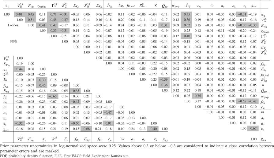Table 2. Elements of the reduced error covariance matrix, equal to the correlation coefficient, derived from the posterior PDF at the FIFE and Loobos sites

There is one important difference between the two sites that affects parameter correlations: for FIFE, canopy conductance is assimilated, whereas for Loobos it is (through latent heat flux) the measured transpiration rate. For example, the correlation between c_w and ɛ_s is 0.91 for FIFE, but –0.12 for Loobos. Also, c_w at Loobos is highly correlated with w_pwp, a parameter that is absent at FIFE. For both sites, increasing c_w leads to a higher root supply rate and an increase in the canopy conductance and transpiration rate, all other parameters being equal. Increasing ɛ_s, through increasing net radiation, increases atmospheric demand (D in the model description, see Appendix), and through this the transpiration rate. As stomata respond to atmospheric demand by closing (Eqn (A17)), increasing ɛ_s, leads to a decrease in canopy conductance. To match the quantity that is assimilated, both c_w (or w_pwp) and ɛ_s have either opposing effects (FIFE: on canopy conductance) and are correlated, or have an effect that goes in the same direction (Loobos: on transpiration) and must therefore be anticorrelated to compensate each other.

Analysis of the posterior PDF

So far, we have only analyzed means and covariances derived from the PDF of the posterior parameters. Table 3 lists the prior and posterior means of both the model and the log-normalized parameters. We will now assess whether the assumption of Gaussian posterior distributions is adequate – the advantage would be easy use of the PDF in a global CCDAS (see Introduction). The analysis is based on the medium case of 0.25 prior uncertainty of log-normalized parameters. The skewness and kurtosis of the PDF projected onto each log-normalized parameter is also listed in Table 3. Skewness measures whether a distribution is ‘leaning,’ or skewed, towards either the left (i.e. values smaller than the mean, negative skewness), or the right (positive skewness). Kurtosis indicates ‘peakedness’ relative to a Gaussian distribution, where distributions flatter than Gaussian have negative values (Storch & Zwiers, 1999). Most parameters show only small deviations from a Gaussian distribution, with skewness often slightly negative.

A few parameters, however, are more negatively skewed and some have a markedly ‘pointed’ distribution (high positive kurtosis): ɛ for FIFE, and E_Vm, g_a,v and w_pwp for Loobos (see Fig. 4). E_Vm, g_a,v also show an increase in the standard deviation from prior to posterior. If the distribution of a parameter is much different from Gaussian, then estimation techniques that use the gradient in parameter space to find the cost function minimum, and second derivatives of the cost function to derive parameter uncertainties, will give erroneous results. For f_Ci (FIFE), this would lead to a mean of 1.11 instead of 1.09, and a slight underestimate of the uncertainty. The effect would not be large for w_pwp (Loobos), either, and still quite acceptable for g_a,v, given the generally large uncertainties.

Extrapolation of results in time

We have obtained a constrained parameter PDF for the BETHY C4 and C3 models from 4 or 7 selected days of eddy covariance data, respectively. The question to ask now is how the gained process knowledge, expressed through reduced parameter uncertainty, translates into reduced uncertainty about the quantity of highest interest: the net sink at the site over a longer time period. For that purpose, we have computed the cumulative NEE over a period of 2 years at the Loobos site, complete with 95% confidence ranges, from the prior, the posterior Gaussian, and the full-posterior PDF. The posterior Gaussian PDF approximates the full PDF by using only the means and the error covariance matrix. As Fig. 5 shows by the green area, prior uncertainties about parameter values of BETHY were consistent with the Loobos site being both a strong sink (positive NEE), or a moderate source of carbon (negative NEE) over the 2 years. After constraining the model, the 95% confidence range lies outside of the median prior estimate and Loobos is now very definitely identified as a CO₂ sink. This means that extrapolating 7 days of NEE and LE data through the assimilation procedure resulted in a sink estimate that was both significantly different from the best prior estimate and significantly different from zero. Further, we find that using the full PDF in parameter space results in only about half of the uncertainty in NEE over the 2 years compared with using a PDF derived from parameter means and covariances. Skewness and kurtosis of the full PDF of the cumulative NEE can also be relatively large.

Note that this result still depends on the prior uncertainty, which was only estimated in a simple and preliminary way for this study. Also, assimilating more days of flux measurements would lead to stronger constraints of model parameters and fluxes, which would lead to even smaller uncertainties of the cumulative NEE. Here, we can instead use the measured NEE of the 2 years, with a few gaps (for which we assumed NEE=0), to validate our time extrapolation (Fig. 5, blue line). With this additional assumption as a point of caution, we arrive at around 25 mol(CO₂) m⁻² yr⁻¹ or 300 g C m⁻² yr⁻¹ net uptake from both the observations and the model simulations. The generally good agreement between modeled (after assimilation) and measured NEE across the 2 years shows that the model is able to capture the main processes that influence this quantity. We therefore suggest, that the method shown here with all available measurements assimilated, could be a superior gap filling method compared with the ones usually employed by the eddy covariance community.

Discussion

We have performed several Bayesian inversions of an ecosystem model, BETHY, constrained by eddy covariance data of carbon and water fluxes. There were two sites, one C3 and one C4, and three sets of assumptions about prior parameter uncertainties. We find that the method works very well, although some care has to be taken to insure algorithm convergence. Compared with non-Bayesian, standard optimization techniques (e.g. Wang et al., 2001), the method treats all parameters equally and simultaneously, and is still able to distinguish between those parameters that can be constrained by the eddy covariance data, and those that cannot. With 4 or 7 days of diurnal data assimilated, the Bayesian part of the cost function in the region of the minimum was between two and 10 times the cost of the measurements, so that the inversion was found to be constrained predominantly by the flux data. Similar to Wang et al. (2001), who used non-Bayesian inversions, we find that typically five parameters can be effectively constrained by the method. Perhaps not surprisingly, two to three of them are stomatal parameters: stomata control the balance between carbon uptake and transpiration at the leaf level, both were assimilated, albeit at the stand level. This shows that leaf-level functional representations can be effectively constrained. One of the parameters, ɛ_s, strictly speaking, belongs to the external driver of BETHY used in the computation of incoming thermal radiation. This particular result indicates that assimilating accurate radiation data (obliterating the need for ɛ_s) will likely improve parameter estimation further. We could also constrain parameters describing the light response (α_i, α_q), and sometimes the temperature response of photosynthesis (k²⁵). It is evident that a sufficient range of environmental conditions must be present during the period for which the data were assimilated to gain information about the dependencies on those conditions. The use of a diurnal cycle and of different dates across the seasons must have helped here, and may explain how well the eddy-flux constrained model performed against the 2-year measurements.

The method also delivers information on the error covariances of parameters. This information can be used to find out which processes can be constrained individually by the assimilation of the eddy flux data. Analysis of the full PDF, only possible by Monte Carlo methods, shows that most parameters tend to have distributions close enough to a Gaussian one for gradient and second-derivative methods to work effectively. These usually require a few orders of magnitude fewer iterations. Only one parameter was identified with a distribution so far away from a normal one that such methods would have underestimated the posterior mean and uncertainty to a large degree.

One straightforward and easy application of the method presented here would be to use the posterior means and covariances of the parameter PDF as priors in a global-scale data assimilation system (cf. Rayner et al., 2005). We expect that using the Gaussian part of the complete PDF will tend to overestimate the uncertainty of the model diagnostics.

We have found that the results of our study depended on the prior uncertainty of the parameter values. This uncertainty itself will depend on the parameter in question, the scale at which the model is applied, and the amount of available information at that scale. Our preliminary results (unpublished) indicate that for V_m²⁵, 0.5 prior uncertainty at the site scale would be a realistic assumption in the log-normalized space if only the functional type of vegetation is known.

We have so far restricted our study to cases that are rather rare when considering the entire FLUXNET archive: we relied on the availability of soil moisture measurements. Applying the method for more sites, however, will be crucial for identifying representative model parameterizations by plant functional type, or some other generalization on which global models necessarily rely. Therefore, we expect to conduct further studies using the complete BETHY model with the full water balance. If no complete data on LAI are available, a phenology scheme may also be included. LAI and soil moisture data could then also be assimilated instead of being used as input. We also suggest using more days and longer periods for assimilation, although we find that only a few days of data already deliver a strong model constraint.

Conclusions

The parameterization of global TEMs for carbon cycle studies poses great challenges. We are confronted with model errors, errors from the finite accuracy of parameter estimation, and representation errors that result from the fact that models need to work with a finite set of idealized vegetation types. This study demonstrates that inversion against eddy covariance data can be a powerful tool for using local measurements to constrain the possible range of ecosystem model parameters. Such information about parameter uncertainties is crucial for understanding to what degree of confidence we can use models to compute the global terrestrial carbon balance.

The advantage of the Monte Carlo inversion technique is that it works even for highly nonlinear models, and that it allows sampling the complete posterior PDF. This can be used to estimate how well methods will work that derive uncertainties from the curvature of the cost function at its global minimum. Because they require far fewer iterations, such methods are better suited for global applications, especially when parameters need to be inverted simultaneously.

Further use of this method will require a careful analysis of the prior uncertainties of model parameters. For the envisaged global applications, it will also be important to repeat the analysis with a sufficient number of sites per major vegetation type in order to gain an understanding of the representation error. We suggest that using such studies to determine prior parameter uncertainties for global carbon cycle data assimilation could be one of the principle applications of data from the growing network of eddy covariance measurement sites. We believe that such a method of extrapolating measurements from local sites to the global scale through the determination and spatial extrapolation of parameters would be the most promising and most adequate route to better global TEMs. These will be crucial for any application aimed at predicting the future response of the carbon cycle to climate change, including atmosphere – vegetation feedbacks.

Acknowledgments

The original eddy flux data used in this study were collected, maintained and generously provided by Eddy Moors, Jan Elbers, Wilma Jans, Han Dolman and colleagues affiliated with the Loobos Research Site in The Netherlands, run by ALTERRA, Green World Research. The authors wish to thank Bart Kruijt and Isabel van den Wyngaert for help with estimating uncertainties of eddy covariance measurements and Thomas Kaminski for useful advice and comments. This work has been financed and supported by the EU project CAMELS, contract number EVK2-CT-2002-00151, within the EU's 5th framework program for Research and Development, and the Max-Planck-Gesellschaft zur Förderung der Wissenschaften, e.V.

Appendix

Appendix: The BETHY model

Overview

We use a process-based model of the coupled photosynthesis and energy balance system, the BETHY scheme, to simulate the exchange of CO₂, water and energy between the plant canopy and the atmosphere. BETHY computes absorption of PAR in three layers, while the canopy air space is treated as a single, well mixed air mass with a single temperature. Evapotranspiration and sensible heat fluxes are calculated from the Penman–Monteith equation (Monteith, 1965). Carbon uptake is computed with the model by Farquhar et al. (1980) for C3, and the one by Collatz et al., (1992) for C4 plants. The stomata and canopy model of Knorr (2000) simulates canopy conductance in response to PAR; in the absence of water stress in such a way as to satisfy the demand for CO₂. In water-stressed situations, stomata are further closed until transpiration reaches a specific root supply rate that depends on soil moisture. The carbon balance is computed as plant and soil respiration subtracted from the photosynthesis rate to yield net CO₂ fluxes. The full version of BETHY, described in Knorr (2000) and Knorr and Heimann (2001a), also contains submodels for soil water balance, snow, canopy and soil evaporation, and phenology, which are not used here. Instead, LAI and soil moisture are treated as external forcing data (elements of s in Eqn (1)). The version of BETHY for C3 vegetation used here has 23 free parameters, while the C4 version has 14. Following is a description of all free model parameters and their meaning in the context of the model. Parameters have been marked as underlined mathematical symbols and are listed in Table 1, complete with their prior values. (Those that do not appear in one of the equations appear underlined in the text.)

Photosynthesis

For C3 vegetation, gross leaf CO₂ uptake, A, is calculated as (cf. Farquhar et al., 1980):

((A1a))

with

((A1b))

((A1c))

A is gross photosynthesis, or GPP, I is absorbed PAR, C_i the leaf-internal CO₂, and O_x the oxygen concentration (=0.21 mol(O₂)/mol(air)). α_q is the quantum efficiency of photon capture (mol(e⁻) mol(photons)⁻¹) and V_m the maximum carboxylation rate (in mol(CO₂)m⁻² s⁻¹), expressed as

((A2))

with the activation energy E_Vm (in J mol⁻¹). Λ_u and Λ_l are the LAI of the upper and lower bounds of the specific canopy layer under consideration, and k₁₂ a leaf nitrogen scaling parameter set to 0.5/cos(θ₁₂). θ₁₂ is the solar zenith angle at noon.

Further, J_m, the maximum electron transport rate (same units as V_m), is expressed as

((A3))

This rate, at standard temperature, is assumed proportional to V_m with an additional proportionality constant (e.g. Wullschleger, 1993). T_c is the canopy temperature in °C, T_k the canopy temperature in Kelvin, and R the universal gas constant (8.314 J K⁻¹ mol⁻¹). The CO₂ compensation point without dark respiration, Γ_*, follows from:

((A4))

The two Michaelis–Menten constants for carboxylation and oxygenation, K_C and K_O, respectively (in J mol⁻¹), have a temperature dependence based on Arrhenius' equation similar to V_m:

((A5))

and

((A6))

For C4 photosynthesis, the model of Collatz et al. (1992) is used with:

((A7a))

with

((A7b))

((A7c))

((A7d))

V_m is computed from Eqn (A2), α_i is the C4 quantum efficiency (in mol(CO₂)/mol(photons)), and k is the C4 CO₂ specificity (in mol(CO₂) m⁻² s⁻¹), with

((A8))

Photosynthesis rates are computed across three different layers of the canopy, each with its own value for I and V_m, and thus A. The sum over the three layers yields A_c, the canopy gross photosynthesis.

Carbon balance

To compute net CO₂ uptake by the leaves, leaf or ‘dark’ respiration, R_d, is subtracted from A to yield net leaf CO₂ uptake, A_n, with

((A9))

and

((A10))

Summation of R_d across canopy layers yields R_d,c, the canopy dark respiration.

There are two standard values for f_Rd, one for C3 and one for C4 vegetation. Dark respiration is assumed to be a constant fraction of total plant, or autotroph respiration, R_aut, such that

((A11))

f_R,leaf stands for the fraction of total plant respiration contributed by the leaves. This formulation differs from the form chosen in the original description of BETHY, which contains an additional term for ‘growth respiration’ assumed proportional to net primary productivity. Such an implicit formulation yields a sum of two terms, one of which is proportional to R_aut of Eqn (A10), the other to GPP. The above formulation was chosen for simplicity in order to avoid unnecessary co-dependence of parameters.

For soil (excluding root), or heterotroph respiration, R_het, we use an exponential temperature dependence on air temperature (T_a, in °C) times a soil water factor (with zero respiration at zero plant-available soil moisture):

((A12))

w_m is the plant available soil water content at field capacity (% volume), and R_het⁰ soil respiration at 0°C and with soil water content at field capacity. w is the plant-available soil water content (% volume) and is computed from total soil moisture, w_tot, as w=max{w_tot, w_m}−w_pwp, is the soil water content at the permanent wilting point, which is used as another free parameter in the case that total soil water content is used as input.

Finally, the net carbon flux of the site is given by

((A13))

Stomatal control

The model of stomatal control follows the assumption that, in the absence of water stress, leaf-level photosynthesis operates at a standard ratio between the leaf-internal CO₂ concentration, C_i, and the CO₂ concentration of free air, C_a. This value is given by

((A14))

with two values for f_Ci, one for C3 and one for C4 vegetation. In order to determine the demand for CO₂ uptake, A_n is first calculated as A_n,0 for C_i=C_i,0, and T_c=T_a. Inversion of the diffusion equation for CO₂ at the stomatal boundary is then used to compute stomatal conductance in the absence of water stress at each canopy layer (in m s⁻¹):

((A15))

p is air pressure (in Pa). If at the time of highest demand, D, transpiration rates exceed a root water supply rate, S, stomatal conductance at each canopy layer is reduced according to

((A16))

by adjusting b_e such that S=D. D_a is the VPD of the free air. This supply rate is taken as

((A17))

Next, the canopy temperature, T_c, is computed consistent with the energy balance after integrating g_s over the canopy to obtain the canopy conductance used in the Penman–Monteith equation. Then, the photosynthesis model is run again, but at a fixed stomatal conductance, g_s, obtained from Eqn (A16), which yields the final gross, A, and net photosynthesis rate, A_n.

Energy and radiation balance

PAR absorption is calculated according to the two-flux scheme by Sellers (1985) with three vertical layers of equal LAI. The diffuse fraction of PAR is calculated according to a procedure by Weiss and Norman (1985). Leaf-angle distribution is assumed to be uniform, and the only free parameters for this scheme is ω, the leaf single-scattering albedo.

To determine evapotranspiration rates from the Penman–Monteith formula, BETHY computes net radiation balance of the canopy, R_n,c, according to the following equation:

((A18))

ɛ_a and ɛ_sfc=0.97 are sky and surface emissivity, respectively, T_K,a air temperature in Kelvin, σ=5.6703 × 10⁻⁸ W m⁻² K⁻⁴ the Stefan–Boltzmann constant, and t_l,v the longwave transmissivity of the vegetation, assumed t_l,v=f_c exp(−0.5Λ/f_c)+(1−f_c). f_c is the fraction of soil covered by vegetation. For the shortwave part, R_S is incoming solar radiation (W m⁻²), f_PAR is the fraction of PAR absorbed by the vegetation and computed by the two-flux scheme, a_v the albedo of the vegetation at the limit of high LAI and closed canopy, and a_s the amount of solar radiation absorbed by the soil under the canopy at the same limit. G is the ground heat flux, assumed to be a fixed fraction of total net radiation. (Contrary to R_n,c, total net radiation does not depend on G, so there is no implicit equation to be solved.) The sky emissivity is computed from

((A19))

with the cloud cover fraction n_c. If no separate radiation data for PAR and solar radiation are available, R_S is calculated from PAR according to Weiss and Norman (1985).

The aerodynamic exchange between the canopy and the free air is described as

((A20))

with wind speed, u, and a proportionality factor serving as a free model parameter. Wind speeds below 1 m s⁻¹ are uniformly set to 1 m s⁻¹ to avoid unrealistically high canopy temperature under conditions of extremely still air and high incoming radiation. The prior value of g_a,v is determined from the following formula:

((A21))

h_ref is the reference height above canopy (10 m), h_c the canopy height, k=0.41, r_z=0.1 and a_z=1.

References

Collatz GJ, Ribas-Carbo M, Berry JA (1992) Coupled photosynthesis–stomatal conductance model for leaves of C4 plants. Australian Journal of Plant Physiology, 19, 519–538.
10.1071/PP9920519
Web of Science® Google Scholar
Cowles MK, Carlin BP (1996) Markov chain Monte Carlo convergence diagnostics: a comparative review. Journal of the American Statistical Association, 91, 883–904.
10.1080/01621459.1996.10476956
Web of Science® Google Scholar
Cox PM, Betts RA, Jones CD et al. (2000) Acceleration of global warming due to carbon-cycle feedbacks in a coupled climate model. Nature, 408, 184–187.
10.1038/35041539
CAS PubMed Web of Science® Google Scholar
Cramer W, Kicklighter DW, Bondeau A et al. (1999) Comparing global models of terrestrial net primary productivity (NPP): overview and key results. Global Change Biology, 5 (Suppl. 1), 1–15.
10.1046/j.1365-2486.1999.00009.x
Web of Science® Google Scholar
Cramer W, Bondeau A, Woodard FI et al. (2001) Global response of terrestrial ecosystem structure and function to CO₂ and climate change: results from six dynamic global vegetation models. Global Change Biology, 7, 357–373.
10.1046/j.1365-2486.2001.00383.x
Web of Science® Google Scholar
Dolman AJ, Moors EJ, Elbers JA (2002) The carbon uptake of a mid latitude pine forest growing on sandy soil. Agricultural and Forest Meteorology, 157–170.DOI: 10.1016/S0168-1923(02)00024-2
10.1016/S0168-1923(02)00024-2
Web of Science® Google Scholar
Farquhar GD, Von Caemmerer S, Berry JA (1980) A biochemical model of photosynthesis in leaves of C3 species. Planta, 149, 78–90.DOI: 10.1007/BF00386231DOI: 10.1029/94JB03097DOI: 10.1029/94JB03097
10.1007/BF00386231
CAS PubMed Web of Science® Google Scholar
Friedlingstein P, Dufresne JL, Cox PM et al. (2003) How positive is the feedback between climate change and the carbon cycle? Tellus, 55B, 692–700.
10.1034/j.1600-0889.2003.01461.x
CAS Web of Science® Google Scholar
Gelman A, Carlin JB, Stern HS et al. (1995) Bayesian Data Analysis. Chapman and Hall/CRC, New York.
10.1111/j.1574-6941.2001.tb00841.x
CAS PubMed Web of Science® Google Scholar
Gelman A, Rubin DB (1992) A single squence from the Gibbs sampler gives a false sense of security. In: Bayesian Statistics (eds JM Bernardo, JO Berger, AP Dawid, AFM Smith), pp. 625–631. Oxford University Press, Oxford.
Google Scholar
Global Carbon Project (2003) Science Framework and Implementation. Global Carbon Project, Earth System Science Partnership (IGBP, IHDP, WCRP, DIVERSITAS), Canberra.
Google Scholar
Joos F, Plattner GK, Stocker TF et al. (2003) Trends in marine dissolved oxygen: implications for ocean circulation changes and the carbon budget. EOS, 84, 197–201.
10.1029/2003EO210001
Google Scholar
Kaminski T, Knorr W, Heimann M et al. (2002) Assimilating atmospheric data into a terrestrial biosphere model: a case study of the seasonal cycle. Global Biogeochemical Cycles, 16, 1066 (doi: 10.1029/2001GB001463).DOI: 10.1029/2001GB001463
10.1029/2001GB001463
CAS Web of Science® Google Scholar
Kim J, Verma SB (1991) Modeling canopy photosynthesis: scaling up from a leaf to canopy in a temperate grassland ecosystem. Agricultural and Forest Meteorology, 57, 149–166.DOI: 10.1016/0168-1923(91)90028-O
10.1016/0168-1923(91)90028-O
Web of Science® Google Scholar
Knorr W (1997) Satellite Remote Sensing and Modelling of the Global CO₂ Exchange of Land Vegetation: A Synthesis Study. Max-Planck-Institut für Meteorologie, Hamburg, Germany.
Google Scholar
Knorr W (2000) Annual and interannual CO₂ exchanges of the terrestrial biosphere: process-based simulations and uncertainties. Global Ecology and Biogeography, 9, 225–252.DOI: 10.1046/j.1365-2699.2000.00159.x
10.1046/j.1365-2699.2000.00159.x
Web of Science® Google Scholar
Knorr W, Heimann M (2001a) Uncertainties in global terrestrial biosphere modeling. Part I: a comprehensive sensitivity analysis with a new photosynthesis and energy balance scheme. Global Biogeochemical Cycles, 15, 207–225.DOI: 10.1029/1998GB001059
10.1029/1998GB001059
CAS Web of Science® Google Scholar
Knorr W, Heimann M (2001b) Uncertainties in global terrestrial biosphere modeling. Part II: global constraints for a process-based vegetation model. Global Biogeochemical Cycles, 15, 227–246.DOI: 10.1029/1998GB001060
10.1029/1998GB001060
CAS Web of Science® Google Scholar
Leuning R (2002) Temperature dependence of two parameters in a photosynthesis model. Plant, Cell and Environment, 25, 1205–1210.DOI: 10.1046/j.1365-3040.2002.00898.x
10.1046/j.1365-3040.2002.00898.x
CAS Web of Science® Google Scholar
McGuire AD, Sitch S, Clein JS et al. (2001) Carbon balance of the terrestrial biosphere in the twentieth century: analyses of CO₂, climate and land use effects with four process-based ecosystem models. Global Biogeochemical Cycles, 15, 183–206.DOI: 10.1029/2000GB001298
10.1029/2000GB001298
CAS Web of Science® Google Scholar
Medlyn BE, Loustau D, Delzon S (2002) Temperature response of parameters of a biochemically based model of photosynthesis. I. Seasonal changes in mature maritime pine (Pinus pinaster Ait.). Plant, Cell and Environment, 25, 1155–1165.DOI: 10.1046/j.1365-3040.2002.00890.x
10.1046/j.1365-3040.2002.00890.x
CAS Web of Science® Google Scholar
Metropolis N, Rosenbluth AW, Rosenbluth MN et al. (1953) Equation of state calculations by fast computing machines. Journal of Chemical Physics, 21, 1087–1092.DOI: 10.1063/1.1699114
10.1063/1.1699114
CAS PubMed Web of Science® Google Scholar
Monteith JL (1965) Evaporation and environment. Symposium of the Society for Experimental Biology, 19, 205–234.
CAS PubMed Google Scholar
Mosegaard K (1998) Inverse problems. Inverse Problems, 14, 405–426.DOI: 10.1088/0266-5611/14/3/004
10.1088/0266-5611/14/3/004
Web of Science® Google Scholar
Mosegaard K, Rygaard-Hjalsted C (1999) Probabilistic analysis of implicit inverse problems. Inverse Problems, 15, 572–583.
10.1088/0266-5611/15/2/015
Web of Science® Google Scholar
Mosegaard K, Sambridge M (2002) Monte Carlo analysis of inverse problems. Inverse Problems, 18, R29–R54.DOI: 10.1088/0266-5611/18/3/201
10.1088/0266-5611/18/3/201
Web of Science® Google Scholar
Mosegaard K, Tarantola A (1995) Monte Carlo sampling of solutions to inverse problems. Journal of Geophysical Research, 100, 12431–12447.
10.1029/94JB03097
Web of Science® Google Scholar
Prentice IC, Farquhar GC, Fasham MJR et al. (2001) The carbon cycle and atmospheric carbon dioxide. In: Climate Change 2001: The Scientific Basis. Contribution of Working Group I to the Third Assessment Report of the Intergovernmental Panel on Climate Change (eds JT Houghton et al.), pp. 185–225. Cambridge University Press, Cambridge.
Google Scholar
Raich JW, Potter CS, Bhagawati D (2002) Interannual variability in global soil respiration, 1980–94. Global Change Biology, 8, 800–812.DOI: 10.1046/j.1365-2486.2002.00511.x
10.1046/j.1365-2486.2002.00511.x
Web of Science® Google Scholar
Rayner PJ, Scholze M, Knorr W et al. (2005) Two decades of terrestrial carbon fluxes from a Carbon Cycle Data Assimilation System (CCDAS). Global Biogeochemical Cycles (in press).
10.1029/2004GB002254
CAS Web of Science® Google Scholar
Reichstein M, Rey A, Freibauer A (2003) Modeling temporal and large-scale spatial variability of soil respiration from soil water availability, temperature and vegetation productivity indices. Global Biogeochemical Cycles, 17, 1104 (doi:10.1029/2003GB002035).DOI: 10.1029/2003GB002035
10.1029/2003GB002035
Web of Science® Google Scholar
Schachtschabel P, Blume HP, Bruemmer G et al. (1992) Lehrbuch der Bodenkunde. Ferdinand Enke Verlag, Stuttgart.
Google Scholar
Sellers PJ (1985) Canopy reflectance, photosynthesis and transpiration. International Journal of Remote Sensing, 6, 1335–1372.
10.1080/01431168508948283
Web of Science® Google Scholar
V. Storch H, Zwiers FW (1999) Statistical Analysis in Climate Research. Cambridge University Press, Cambridge, UK.
10.1017/CBO9780511612336
Google Scholar
Wang YP, Leuning R, Cleugh H et al. (2001) Parameter estimation in surface exchange models using nonlinear inversion: how many parameters can we estimate and which measurements are most useful? Global Change Biology, 7, 495–510.DOI: 10.1046/j.1365-2486.2001.00434.x
10.1046/j.1365-2486.2001.00434.x
Web of Science® Google Scholar
Weiss A, Norman JA (1985) Partitioning solar radiation into direct and diffuse, visible and near-infrared components. Agricultural and Forestry Meteorology, 34, 205–213.DOI: 10.1016/0168-1923(85)90020-6
10.1016/0168-1923(85)90020-6
Web of Science® Google Scholar
White MA, Thornton PE, Running SW et al. (2000) Parameterization and sensitivity analysis of the BIOME–BGC terrestrial ecosystem model: net primary production controls. Earth Interactions, 4, 1–85.DOI: 10.1175/1087-3562(2000)004<0003:PASAOT>2.0.CO;2
10.1175/1087-3562(2000)004<0003:PASAOT>2.0.CO;2
Google Scholar
Wullschleger SD (1993) Biochemical limitations to carbon assimilation in C3 plants – a retrospective analysis of the A/c_i curves from 109 species. Journal of Experimental Botany, 44, 907–920.
10.1093/jxb/44.5.907
CAS Web of Science® Google Scholar

Citing Literature

Volume11, Issue8

August 2005

Pages 1333-1351

Inversion of terrestrial ecosystem model parameter values against eddy covariance measurements by Monte Carlo sampling

Abstract

Introduction