Beyond the visible: Accounting for ultraviolet and far-red radiation in vegetation productivity and surface energy budgets
Abstract
Photosynthetically active radiation (PAR) is typically defined as light with a wavelength within 400–700 nm. However, ultra-violet (UV) radiation within 280–400 nm and far-red (FR) radiation within 700–750 nm can also excite photosystems, though not as efficiently as PAR. Vegetation and land surface models (LSMs) typically do not explicitly account for UV's contribution to energy budgets or photosynthesis, nor FR's contribution to photosynthesis. However, whether neglecting UV and FR has significant impacts remains unknown. We explored how canopy radiative transfer (RT) and photosynthesis are impacted when explicitly implementing UV in the canopy RT model and accounting for UV and FR in the photosynthesis models within a next-generation LSM that can simulate hyperspectral canopy RT. We validated our improvements using photosynthesis measurements from plants under different light sources and intensities and surface reflection from an eddy-covariance tower. Our model simulations suggested that at the whole plant level, after accounting for UV and FR explicitly, chlorophyll content, leaf area index (LAI), clumping index, and solar radiation all impact the modeling of gross primary productivity (GPP). At the global scale, mean annual GPP within a grid would increase by up to 7.3% and the increase is proportional to LAI; globally integrated GPP increases by 4.6 PgC year−1 (3.8% of the GPP without accounting for UV + FR). Further, using PAR to proxy UV could overestimate surface albedo by more than 0.1, particularly in the boreal forests. Our results highlight the importance of improving UV and FR in canopy RT and photosynthesis modeling and the necessity to implement hyperspectral or multispectral canopy RT schemes in future vegetation and LSMs.
1 INTRODUCTION
Global average surface temperature has increased by around 1.1°C compared to the pre-industrial era primarily due to anthropological CO2 emissions (IPCC, 2023), quickly approaching the 2°C goal settled in the Paris Agreement. Concerted climate actions have been taken and proposed to reduce greenhouse gas emissions and to increase carbon capture (e.g., Liu et al., 2021; Williams et al., 2021). The land system sequesters about 25% of anthropogenic CO2 emission (Friedlingstein et al., 2023), and therefore maintaining or enhancing the terrestrial carbon sink strength is crucial for meeting the carbon neutralization goals. On the one hand, vegetation serves as a potential carbon sink to remove the greenhouse gas CO2 from the atmosphere through photosynthesis and promotes evapotranspiration thus lowering the surface temperature. On the other hand, vegetation takes up radiation energy which could otherwise be reflected by soil and snow. Therefore, to more systematically assess the impact of vegetation on terrestrial carbon, water, and energy fluxes requires more accurate modeling of the surface processes in a coupled system. Meanwhile, this helps predict endangered ecosystems from climatic disasters, such as rare drought stress and wildfire (Anderegg et al., 2015, 2016; Choat et al., 2018; Westerling et al., 2006), being useful to inform policymakers to take action beforehand.
Terrestrial plant photosynthesis is mostly powered by photons with wavelengths within 400–700 nm, known as photosynthetically active radiation (PAR, see Table 1 for the list of symbols). The primary reasons are (1) ultra-violet (UV) with wavelength <400 nm that could damage the photosystems I and II (PSI and PSII) is mostly absorbed by protective materials such as flavonoids and cellulose (Markham & Mabry, 1975) and (2) isolated chlorophylls and carotenoids, which are the main pigments in PSI, PSII, and light harvest complexes (LHCs) (Gao et al., 2018; Mazor et al., 2015; Sheng et al., 2018; Wei et al., 2016), are barely found to absorb photons with wavelength >700 nm (Cinque et al., 2000; Lichtenthaler, 1987; Lichtenthaler & Buschmann, 2001; Linschitz & Sarkanen, 1958; Peters & Noble, 2014). However, the peripheral LHCs of PSI are found to absorb a small amount of far-red (FR) radiation photons with 700–750 nm wavelength (Croce & Van Amerongen, 2013; Wientjes & Croce, 2011), thus boosting photosynthesis when used along with PAR (Zhen & Bugbee, 2020a). Therefore, a small portion of UV and FR could be absorbed by the photosystems and further contribute to photosynthesis, but vegetation and land surface models (LSMs) often did not explicitly take them into account.
| Symbol | Description |
|---|---|
| ASTM | American society for testing and materials |
| CLM | Community land model |
| CliMA Land | Land model developed within climate modeling alliance |
| ESM | Earth system model |
| FR | Far-red radiation (wavelength: 700–750 nm) |
| LHC | Light harvest complex |
| LSM | Land surface model |
| NIR | Near infrared radiation (wavelength 700–2500 nm) |
| PAR | Photosynthetically active radiation (wavelength: 400–700 nm) |
| PFT | Plant functional type |
| PROSPECT | Leaf optical properties spectra model |
| PSI | Photosystem I |
| PSII | Photosystem II |
| RMSE | Root mean squared error |
| RT | Radiative transfer |
| SCOPE | Soil canopy observation, photochemistry, and energy fluxes model |
| SPAC | Soil–plant–air continuum |
| UV | Ultraviolet radiation (wavelength: 280–400 nm) |
| A g | Gross photosynthetic rate |
| CHL | Chlorophyll content |
| CI | Clumping index |
| g s | Stomatal conductance to water vapor |
| LAI | Leaf area index |
| J max | Maximum electron transport rate at leaf temperature |
| J max25 | Maximum electron transport rate at 25°C |
| V cmax25 | Maximum carboxylation rate at 25°C |
| GPP | Gross primary productivity |
| PPAR | Photons absorbed by chlorophyll used for photosynthesis (280–750 nm) |
| RAD | Radiation |
| SIF | Solar-induced chlorophyll fluorescence |
| SW out | Outgoing shortwave radiation |
| SZA | Solar zenith angle |
According to the American Society for Testing and Materials (ASTM) G-173-03 standard table Reference Air Mass 1.5 Spectra (https://www.nrel.gov/grid/solar-resource/spectra-am1.5.html; last access: 21 February 2024), the land surface on average receives approximately 45.5 W m−2 UV (138.3 μmol m−2 photons; compared to 429.7 W m−2 PAR, 1983.5 μmol m−2 photons). Notably, vegetation and soil have lower surface albedo for UV than PAR; for example, Feister and Grewe (1995) measured the surface albedo at various surfaces and found that plants reflect an average of 2.1% ultra-violet radiation (UV) and 5.7% PAR to the atmosphere among five vegetation types, whereas loam and sand return an average of 12.4% UV and 23.4% PAR to the atmosphere. Despite the substantial UV and PAR surface albedo difference, canopy radiative transfer (RT) models and LSMs tend to neglect the UV or treat it implicitly along with PAR. For example, the SCOPE model (van der Tol et al., 2009; Yang et al., 2017) that simulates hyperspectral canopy RT neglects UV, both for the energy balance and photosynthesis. The broadband canopy RT in the community land model (Lawrence et al., 2019) treats UV and PAR equally as visible light (<700 nm) and uses all the “visible” radiation for photosynthesis. This, however, could also result in biases in the surface energy balance (plants absorb more UV than PAR) and photosynthetic rate (plants use UV less effectively compared to PAR). These biases could potentially propagate to divergences in the global carbon cycle and planetary radiative forcing impacting climate simulations (Braghiere et al., 2023).
Besides, the land surface receives an average of 60.1 W m−2 FR (363.9 μmol m−2 photons), according to the ASTM G-173-03 standard table. Although the canopy RT models and LSMs already account for the FR absorption in their energy balance, they do not explicitly allocate the PSI FR absorption to photosynthesis. As supplementing FR to PAR increases plants' productivity (Zhen & Bugbee, 2020a, 2020b), the way FR is handled in these models could lead to biased modeled photosynthetic rates. Moreover, FR absorption in its wavelength range of 700–750 nm is not as flat as regular near-infrared radiation (NIR) but shows a smooth transition due to the chlorophyll absorption. This smooth transition is accounted for by hyperspectral leaf optics models like PROSPECT (Féret et al., 2017; Jacquemoud et al., 2009; Peters & Noble, 2014) and models based on it, such as SCOPE and CliMA Land (van der Tol et al., 2009; Wang et al., 2021). In comparison, this smooth transition of leaf FR absorption cannot be accurately represented by the broadband canopy RT schemes used in most vegetation models and LSMs as the FR absorption is counted as NIR with constant broadband leaf reflectance and transmittance (Campbell & Norman, 1998; De Pury & Farquhar, 1997; Lawrence et al., 2019; Norman, 1982). In this study, we refer to PAR as the radiation with a wavelength of 400–700 nm and define PPAR as photons absorbed by chlorophyll that are used for photosynthesis (including all the absorbed UV, PAR, and FR photons).
Although monochromatic FR is relatively inefficient for photosynthesis compared to PAR, it shows great potential in agriculture given its enhancement to plant growth (SharathKumar et al., 2020; Slattery & Ort, 2021; Wang & Yin, 2023; Zhen & Bugbee, 2020b). In theory, including FR photons in photosynthesis models would result in higher leaf-level light availability, and thus higher stomatal conductance, higher photosynthetic rates, and shifted photochemical and fluorescence yields (Han et al., 2022; Johnson & Berry, 2021; van der Tol et al., 2014). However, simply counting chlorophyll FR absorption into PPAR could be problematic, because the lower-energy FR photons alone cannot trigger photosynthesis. Research has shown that shorter wavelength photons (below 680 nm) tend to excite PSII whereas longer wavelength photons excite preferentially PSI which requires lower excitation energy (Hogewoning et al., 2012; Laisk et al., 2014), and photosynthesis enhancement is only found when supplementing FR on top of PAR (Emerson & Rabinowitch, 1960; Zhen & Bugbee, 2020a, 2020b). Therefore, the photosynthesis and/or canopy RT models need to be adapted accordingly to distinguish the FR and UV + PAR photons. Otherwise, the models would predict high photosynthetic rates even when plants are under FR only.
In the presented study, we show how we addressed the problems in a next-generation land model developed within the Climate Model Alliance (CliMA Land) in the following aspects. (1) We extended the hyperspectral RT model to include UV with the wavelength of 300–400 nm (which covered the majority of UV energy). (2) We accounted for FR absorbed by chlorophyll in photosynthesis models. (3) We revised the photosynthesis and RT models to distinguish FR and UV + PAR photons. We ask the following: (1) how modeled canopy RT, surface energy budget, and photosynthesis change when implementing these new features, (2) how the canopy integrated photosynthesis differs with various canopy structures and environments, and (3) how global photosynthesis simulations will be impacted. To answer the questions, we first validated our new model features using data collected from plants under different light sources and intensities and from an eddy-covariance tower. We then ran CliMA Land at the site level to perform a theoretical sensitivity analysis of various canopy structures and environmental conditions. We further ran CliMA Land at the global scale to examine the impacts of UV + FR implementations at larger scales.
2 MATERIALS AND METHODS
2.1 CliMA land model
The CliMA Land is a next-generation LSM designed to utilize the increasing number of remote sensing data besides regular carbon and water fluxes (Braghiere et al., 2021; Wang et al., 2021, 2023). The three model design principles of CliMA Land are modularity, user experience, and freedom. CliMA Land is highly modularized so that the interdependencies among the modules can be bypassed when using each module as a standalone package (by prescribing necessary parameters). This enables us to implement the new UV and FR features into CliMA Land with minimum interference with other modules. For a better user experience, CliMA Land is modeled in Julia, which reads like Matlab and Python and runs like C. Users also have the freedom to choose from the alternative schemes we implemented or build their customized schemes using the code loading features of Julia. For example, each CliMA Land module includes a series of alternative model schemes (such as the alternative photosynthesis models we used in the present study), thus allowing for a free combination of compatible models and emulating other LSMs.
CliMA Land is a trait-based model, compared to the traditional LSMs based on plant function type (PFT). For example, when running global simulations, instead of prescribing the trait-independent parameters per PFT, we use plant traits to derive these auxiliary parameters required by the modules such as leaf reflectance and transmittance. The trait-based nature can better account for the spatial and temporal variations of the surface processes. The basic element of the CliMA Land is a soil–plant–air continuum (SPAC), which consists of a vertically resolved soil system, vertical canopy airspace, a plant system (with roots that correspond to the soil layers, trunk, branches, and leaves that correspond to canopy airspace), and environmental conditions (like precipitation and incoming radiation). Per time step, we run the SPAC model in the following steps. (1) We update the auxiliary variables from the state variables. (2) We compute the soil albedo, canopy optical properties based on sun geometry, and canopy shortwave RT, which are not supposed to change in the sub-steps. (3) We use a time stepper function to divide a big time step into multiple sub-steps to avoid numerical issues. Per sub-step, we update the soil water budget, stomatal conductance, photosynthesis, plant water budget, and SPAC energy budget. (4) If the remote sensing features are turned on, we derive canopy optical properties related to sensor geometry and compute canopy reflectance and fluorescence spectra. The prognostic state variables are updated at the end of the time step and will be used for the next time step. All the key parameters of the processes are stored as auxiliary variables in the SPAC structure and can be read or modified anytime during the process.
By default, we run the SPAC model using hyperspectral RT with remote sensing features enabled. Compared to the traditional LSMs, the implementation of the hyperspectral RT schemes in LSMs has allowed new frontiers of research, such as more accurately modeling the surface energy fluxes, running land models with remote sensing features (Norton et al., 2018, 2019), inverting plant traits (Cheng et al., 2020; Croft et al., 2020; Pacheco-Labrador et al., 2019), and emulating satellite observations (Poulter et al., 2022). Although running the complex RT schemes requires more computation resources and model inputs such as leaf pigment concentrations, which do not yet have a mechanistic representation in existing vegetation models, these new features allow us to better learn from data, particularly the increasing number of remote sensing data from multiple satellite platforms. In the present study, we advanced the hyperspectral RT scheme by improving the UV and FR representations. We also revised the photosynthesis models to distinguish the FR and PAR + UV photons.
2.2 UV representation
UV, on average, contributes 45.5 W m−2 to the incoming shortwave radiation of the land surface (Figure 1a). However, the leaf absorption feature per constitute in PROSPECT (e.g., Figure 1b), further adopted by downstream models like SCOPE and CliMA Land, is missing in the UV wavelength range. These absorption features are typically calibrated using the leaf reflectance and transmittance spectra from leaves with measurements of different constitutes (Féret et al., 2017, 2021; Jacquemoud et al., 2009; Jacquemoud & Baret, 1990). However, as the measured leaf spectra barely extend to the UV range, the UV absorption features of the major constituents have not been calibrated in the past (particularly chlorophyll, carotenoid, and leaf dry matter; Figure 1b). Promisingly, the UV absorption features have been reported for extracted chlorophyll (Zhang et al., 2009), carotenoid (Andersson et al., 1991), proteins (Schmid, 2001), and cellulose (Orelma et al., 2020), thus allowing us to extend these absorption features of the major UV absorbers before these UV absorption features being calibrated like PAR and NIR. As the UV within 300–400 nm contains more than 99.99% of the UV energy (ASTM G-173-03 standard table), we only extended the lower boundary from 400 to 300 nm in CliMA Land.
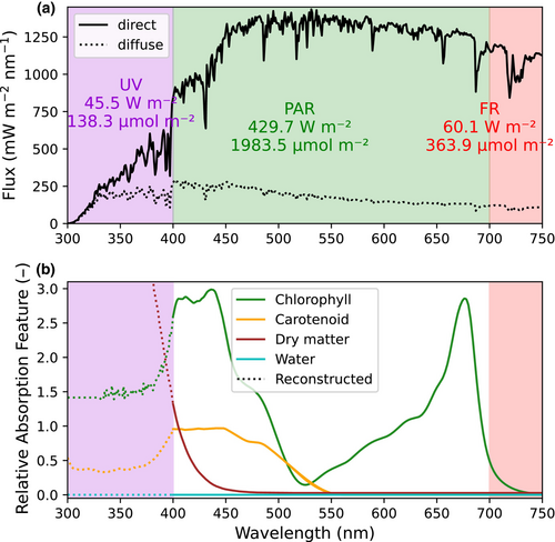
According to Orelma et al. (2020), the UV absorption by cellulose increases linearly with the lower wavelength from 300 to 400 nm. In contrast, the UV absorption by protein only increases substantially with the lower wavelength from 300 to 310 nm (Schmid, 2001). Therefore, in our reconstructed absorption feature of leaf dry matter, we simply linearly extrapolated the PROSPECT curve using the data from 400 to 405 nm (brown dotted curve in Figure 1b). Because of limited knowledge of the UV absorption by other leaf pigments and water, we used the values at 400 nm to represent the unknown UV absorptance (e.g., the cyan dotted curve in Figure 1b plots the extended absorption feature for water). Because of the relatively flat chlorophyll UV absorption coefficient and increasing dry matter UV absorption coefficient with lower wavelength, the chlorophyll absorbs less UV with lower wavelength (Figure S1). However, chlorophyll still contributes a decent amount of UV absorption (7.5% of total absorption at 300 nm and 50% at 400 nm for a leaf with 40 μg cm−2 chlorophyll and 0.012 g cm−2 dry matter; Figure S1).
Compared to the broadband RT scheme that uses constant reflectance and transmittance at PAR to represent those for UV, accounting for UV in photosynthesis modeling is readily doable in the hyperspectral RT scheme. For the present study, we changed the lower bound of the PPAR definition from 400 to 300 nm to include the UV photons absorbed by chlorophyll. As vegetation models and LSMs either completely ignored UV or treated it as PAR, we evaluated the impacts of UV implementation in two experiments. The first experiment was conducted in theory to compare CliMA Land to the models that neglected UV. The second experiment was conducted using flux tower data to compare CliMA Land to the scenario that attributes UV energy to PAR and NIR.
For the first experiment, we ran CliMA Land at the site level using two configurations (one with UV implementation and one without UV implementation) and compared the simulation results at different canopy layers. The simulations were made on a plant with the default setting: leaf area index (LAI) of 3, clumping index (CI) of 1, chlorophyll content (CHL) of 40 μg cm−2 (carotenoid content is 1/7 CHL), leaf mass per area of 0.012 g cm−2, maximum carboxylation rate at 25°C (Vcmax25) of 50 μmol m−2 s−1, maximum electron transport rate at 25°C (Jmax25) of 83.5 μmol m−2 s−1, saturated soil, solar zenith angle (SZA) of 30°, ATSM G-173-03 mean surface solar radiation spectra, air temperature of 25°C, air vapor pressure of 1500 Pa, and atmospheric CO2 concentration of 400 ppm. The stomatal model used was the optimality-based model developed in Wang et al. (2020). We test the UV implementation using two alternative C3 photosynthesis models (Farquhar et al., 1980; Johnson & Berry, 2021).
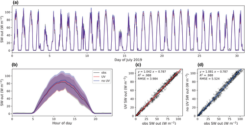
For the second experiment, we ran CliMA Land at the Missouri Ozark flux tower site (MOFLUX) (Gu et al., 2016; Wood et al., 2019) using the prescribed settings: CHL of 57.23 μg cm−2 (carotenoid content is 1/7 CHL), CI of 0.69, LAI of 4, stem area index of 1 (Wang et al., 2021). We ran the model for 2019 July in half-hourly time steps. Per step, we prescribed the total incoming shortwave radiation and soil moisture. SZA was computed using the latitude and local time of the site. For the scenario with UV implementation, we rescaled the radiation spectra from 300 to 2400 nm to match the total incoming shortwave radiation. For the scenario without UV implementation, we set the UV to 0 and rescaled the radiation spectra from 400 to 2400 nm to match the incoming shortwave radiation. We computed and compared the total outgoing shortwave radiation (SW out).
2.3 FR representation
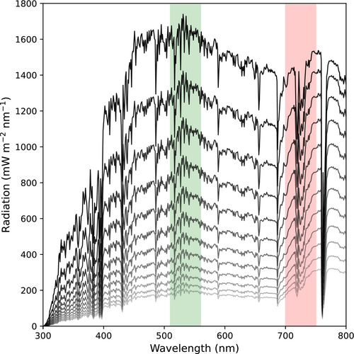
Similar to the UV implementation, accounting for FR in photosynthesis models was done by setting the upper bound of the PPAR definition from 700 to 750 nm. Moreover, as FR was already included in the RT model, counting FR absorption in PPAR does not involve any change in the canopy energy budget. However, due to the higher FR transmittance within the canopy resulting from lower absorptance compared to PAR, the fraction of FR increases in the lower canopy despite the overall decrease in FR. Figure 2 shows examples of radiation spectra at different layers of a canopy; and at the bottom of the canopy, the fraction of FR is even higher than that of green light (Figure 2). In this particular example using natural solar radiation where PAR is abundant, counting FR into PPAR without any change in the photosynthesis model is acceptable because the sum of UV and PAR photons exceeds FR photons.
However, current photosynthesis models are not fully prepared to be used with plants under various light sources, particularly those with high FR fractions. Researchers found that shorter wavelength photons excite preferentially PSII whereas longer wavelength photons excite preferentially PSI (Hogewoning et al., 2012; Laisk et al., 2014), but modelers typically assume that leaf equally partitions the photons between the photosystems. Given that the LHC on PSII may detach and reattach to PSI (Allen et al., 1981), the assumption of equally partitioned photons makes sense when shorter wavelength radiation (below 680 nm) is abundant. However, if the longer wavelength radiation proportion is way higher (e.g., under FR source only), the assumption of equally partitioned photons would be problematic because the LHCs on PSI cannot move to PSII, and thus the modeled PSII electron transport would be overestimated. Therefore, it is essential to partition FR photons from PAR + UV photons in photosynthesis models.
We tested our FR and photosynthesis model improvements using the data collected from Zhen and Bugbee (2020a). We extracted the data for all C3 plants from figures 2–6 of Zhen and Bugbee (2020a), and each data contained a paired measurement of photosynthetic photon flux density and gross primary productivity (GPP). The data points were categorized into three types based on the light sources: far-red LED only, cool white LED only, and combined far-red and cool white LEDs. Note here that the far-red LED contains a small fraction of PAR photons and the cool white LED contains a small fraction of FR photons (figure 1a of Zhen & Bugbee, 2020a). The measurements by Zhen and Bugbee (2020a) were made in an order of high white light only, medium white light only, medium white light in combination with 3–5 far-red light steps from low to high, and medium far-red light only. Therefore, we could partition the PAR and FR photons from the total photons per observation. We also extracted the spectra for the far-red LED and the cool white LED from figure 1 of Zhen and Bugbee (2020a). Then, per observation, we derived the light intensity per LED light source based on the partitioned PAR and FR photons and used the combined spectrum to replace the diffuse light spectrum in CliMA Land (we set the direct light to 0 in our model).
As we did not have physiological traits like Vcmax25 and CHL, per plant, we prescribed LAI provided in Zhen and Bugbee (2020a) but fitted Vcmax25 and CHL by minimizing the mean square error between modeled and measured GPP. We fitted the parameters for both Farquhar et al. (1980) and Johnson and Berry (2021) C3 photosynthesis models while keeping other parameters at their default values. In our simulations, the plant canopy was partitioned into 12 even layers, and each layer had 1/12 of the total LAI. The CHL was set to the constant among all canopy layers, and carotenoid content was assumed to be CHL/7 (Croft et al., 2020). The fitted Vcmax25 was that at the top canopy layer (Vcmax25,top), whereas in the lower canopy layers, Vcmax25 = Vcmax25,top · exp(−0.3 · ΣLAI) (ΣLAI is the cumulative LAI above the canopy layer). Per layer, for the Farquhar et al. (1980) model, the maximum electron transport rate at 25°C was scaled using Jmax25 = 2 · Vcmax25; for the Johnson and Berry (2021) model, cytochrome concentration was scaled using b6f = 0.23 · Vcmax25 [an arbitrary assumption to roughly align the modeled photosynthetic rate to that of Farquhar et al., 1980 model with the same Vcmax25]. We then used the fitted parameters to compute GPPs per plant and compared them to observations to benchmark our revised photosynthesis models.
2.4 Sensitivity analysis
We theoretically evaluated how the improved UV, FR, and photosynthesis representations impact modeled GPP for plants with various traits, structures, and environmental conditions. We varied the following parameters in our sensitivity analysis: CHL, LAI, CI (Chen et al., 2012), and solar radiation. For the sensitivities to CHL, LAI, and CI, we varied only the target parameter while holding others at their default values. For the sensitivity to solar radiation, we used SZA as the primary variable and changed solar radiation accordingly.
CHL impacts the leaf optical properties in UV, PAR, and FR ranges. For the GPP sensitivity to CHL, we ranged CHL from 5 to 80 μg cm−2 with a 5 μg cm−2 step (carotenoid content is CHL/7). Per CHL, we ran CliMA Land on two contrasting configurations (one without UV + FR implementation and one with UV + FR implementation) and then computed the ΔGPP resulting from the implementation of new features. LAI and CI impact the sunlit leaf fraction within different canopy layers and thus incident radiation spectra in the vertical canopy layers. For the sensitivity analysis, we ranged LAI from 0.5 to 8.0 with a 0.05 step. We ranged CI from 0.25 to 1 with a 0.01 step.
In the sensitivity analysis to radiation, we ranged the SZA from 0° to 85° with a 1° step and scaled the default radiation to its cos(SZA)/cos(48.19°) (because the default radiation spectra are modeled using an SZA of 48.19° as in the ASTM G-173-03 standard table). We did not change the diffuse radiation fraction in our simulations. We also tested the case where the solar radiation was scaled to its 2·cos(SZA)/cos(48.19°).
2.5 Global simulations
To assess how the improved UV and FR representations impact global simulations of GPP, we ran CliMA Land at the global scale using two configurations: one with the new improvements enabled and one with these new features disabled. The global simulations were tagged as “a12_gm3”. We configured CliMA Land global simulation using the gridded datasets from GriddingMachine (Wang et al., 2022). The datasets used in the present study (labeled as “gm3”) included soil color (Lawrence & Chase, 2007), soil hydraulic parameters (Dai et al., 2019), canopy height (Simard et al., 2011), CHL (Croft et al., 2020), CI (Wei et al., 2019), LAI (Yuan et al., 2011), specific leaf area (Butler et al., 2017), Vcmax25 (Luo et al., 2021), elevation (Yamazaki et al., 2017), land mask (Hersbach et al., 2020), and plant functional type map used to derive stomatal parameters (Lawrence & Chase, 2007). We refer the readers to https://silicormosia.github.io/blogs/emerald/emerald.html (last access: 13 May 2024) for the detailed benchmark results and logs of CliMA Land global simulations of each simulation version from “a1” to “a12” and from “gm1” to “gm3”.
To further explore how each of CHL (annual mean; reprocessed from Croft et al., 2020), LAI (annual mean; re-gridded from Yuan et al., 2011), and CI (annual mean; re-gridded from Wei et al., 2019) contributes to the change of GPP per grid, we ran the generalized linear model to each of CHL, LAI, and CI using the GLM.jl package (Bates et al., 2023). We further compared our modeled global GPP of the two scenarios against a data-driven GPP product interpolated from flux towers (MPI RS GPP) (Tramontana et al., 2016). The data was labeled as “GPP.RS_V006.FP-ALL.MLM-ALL.METEO-NONE” as noted at https://www.fluxcom.org/CF-Download/. The MPI RS GPP was re-gridded to 1° to match the CliMA Land simulations using the utility tools provided by GriddingMachine.jl (Wang et al., 2022).
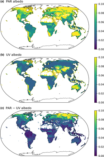
The LSMs within the Earth system models (ESMs) typically use the broadband RT scheme (e.g., Danabasoglu et al., 2020; Golaz et al., 2022; Sellar et al., 2019). These LSMs often use broadband PAR albedo to represent the UV albedo and then pass it back to their coupled atmosphere models, which explicitly include broad UV bands. However, the surface albedo returned by the LSMs may be of great bias because UV albedo is generally lower than PAR albedo (Feister & Grewe, 1995). To assess the magnitude of the bias, we used annual mean CHL re-gridded from Croft et al. (2020) and maximum LAI re-gridded from Yuan et al. (2011) to estimate how the surface albedo of UV may be biased. We ran the canopy RT model per grid using the mean CHL and maximum LAI at one time instant, then computed the mean UV albedo from 300 to 400 nm and mean PAR albedo from 400 to 700 nm per grid for all vegetated grids. Note that the albedo simulation using maximum LAI and mean CHL was meant to roughly estimate the magnitude of the bias in UV surface albedo by broadband models, whereas the time series of LAI and CHL were used in the global simulations.
3 RESULTS
3.1 UV and energy balance
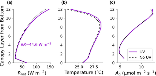
When accounting for a 45.5 W m−2 UV in canopy RT, we found consistently higher net absorbed radiation per canopy layer (the difference decreases in the lower canopy because of the lower UV radiation in the lower layers). The integrated bias was up to 44.6 W m−2 (Figure 3a), corresponding to a UV albedo of 2.0%. As a result, the new version of the model predicted higher leaf and soil temperatures (higher in the upper canopy and topsoil; Figure 3b). However, the photosynthetic rate did not show a detectable difference because most of the UV is absorbed by leaf dry matter (Figure 3c), and the stimulation to photosynthesis and stomatal conductance by the increasing photons is further mitigated by the higher temperature and thus leaf-to-air vapor pressure deficit per canopy layer (Figure 3b). We found similar patterns in the modeled photosynthetic rate when using the Johnson and Berry (2021) C3 (Figure S2).
Our modeled SW out at the flux tower site tracked the observations well in July 2019 for both scenarios with/without UV implementation (Figure 4; R2 = .99 for both scenarios). When averaged to half-hourly means in a diurnal cycle, both scenarios matched the observed mean SW out; the modeled results with UV implementation better agreed with the observations (Figure 4b–d). Notably, the difference between observed and modeled SW out was highest in the noon and afternoon, while the difference was negligible in the morning (Figure 4b). Overall, when implementing UV, the modeled SW out better tracked the observations with a slope closer to 1 and lower root mean squared error (RMSE) (Figure 4c,d).
3.2 FR and photosynthesis
Our modified canopy RT and photosynthesis models could explain the observations that photosynthetic rates increase with supplemental FR to PAR (see black curves in Figure 5a). Further, the model also agreed with the observations that FR alone cannot trigger photosynthesis (see red curves in Figure 5a). For example, the model predicts an elevated GPP when supplementing FR to UV + PAR and a GPP ≈0 under FR only (Figure 5a).
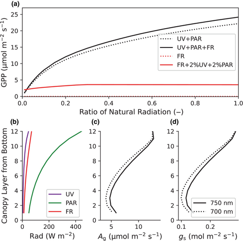
Because FR was already accounted for in the canopy RT model, canopy radiation profiles are not impacted in CliMA Land. Notably, FR has a higher intensity than UV though lower than PAR per canopy layer (Figure 5b). Accounting for FR contribution to PPAR results in higher PPAR photons and thus higher photosynthetic rate per layer, and the increase in photosynthesis is more in lower canopy layers in our shown example (Figure 5c). Further, because of the higher photosynthetic rate, modeled stomatal conductance is also higher per canopy layer (Figure 5d). Note here that the photosynthetic rate and stomatal conductance in the lowest layer were higher than the middle layers, and this was because of the upward reflected solar radiation by the soil, which attenuated from the lowest to the higher canopy layers. We found similar patterns when using the Johnson and Berry (2021) C3 photosynthesis model (Figure S3).
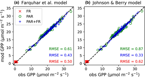
When tested against GPP observations from plants under different light sources and intensities, our revised RT and photosynthesis models well matched the data (Figure 6). Because the far-red LED used in Zhen and Bugbee (2020a) contained a small fraction of PAR photons, the measured and thus modeled GPPs were all slightly higher than 0 when plants were under far-red LED only (red symbols in Figure 6). Our improved photosynthesis models were able to predict the very low GPP; and the RMSEs were 0.50 and 0.62 μmol m−2 s−1, respectively (Figure 6). Similarly, the models also predicted the GPPs under cool white LED only and combined cool white and far-red LEDs with RMSE below 0.9 μmol m−2 s−1 (Figure 6). Overall, the two C3 photosynthesis models performed equally well (with Farquhar et al. (1980) model slightly better), suggesting that our proposed simple PPAR correction to photosynthesis models, namely to partition FR and PAR + UV photons when computing electron transport rate (Equation 7), was working as expected. For the details about the fitting per photosynthesis model, we refer the readers to Figures S4 and S5 for the model-data comparison per plant. As the plants were mostly light-limited, the fitting procedures we used were to fit Jmax25 for the Farquhar et al. (1980) model and b6f for the Johnson and Berry (2021) model, and these fitted parameters per plant showed good linear correlations (Figure S6).
3.3 GPP sensitivity
A higher CHL means that the leaf level UV/PAR/FR absorptance increases and that upper canopy layers absorb more UV/PAR/FR. This, however, will make the FR absorption more valuable to photosynthesis in the lower canopy layers given the higher FR fraction. As a result, it is expected to see ΔGPP increases with higher CHL when CHL is not extremely high. We confirmed this in our simulations that ΔGPP increases with higher CHL when CHL is not extremely high (Figure 7a). There is an extreme case when CHL is too high that the top canopy layers absorb most UV/PAR/FR (e.g., CHL >200 μg cm−2), and further increasing CHL would result in more limited light availability in the lower layers. As the upper layers are typically not light-limited, the higher PPAR values in these layers would not result in higher photosynthesis. Meanwhile, as the lower canopy layers do not have enough photons to power photosynthesis, the ΔGPP would decrease with higher CHL when exceeding a threshold. When we continuously increased CHL in our model, we did find this pattern when CHL exceeds 200 μg cm−2, way beyond the typical range from 10 to 80 μg cm−2 as reported in Croft et al. (2020).

Leaf area index impacts the sunlit leaf fraction and radiation spectra per canopy layer. When not considering soil reflection, a canopy with higher LAI is analogous to treating the canopy as an upper canopy with LAI of l under default solar radiation and a lower canopy with LAI of δl under lower solar radiation (radiation at the lower bound of the upper canopy). Thus, it is expected that ΔGPP increases and eventually saturates with higher LAI (Figure 7b). Like LAI, CI also impacts the sunlit leaf fraction and thus incident radiation spectra. When the canopy is more clumped (lower CI), the sunlit leave fraction (fsunlit) and absorbed radiation in the upper canopy decrease, whereas fsunlit and absorbed radiation in the lower canopy increase. As a result in our example, when CI is higher than 0.72, the impact from increased fsunlit in the lower canopy dominated the simulation, and ΔGPP increased with lower CI; when CI is lower than 0.72 in the example simulation, the impact from decreased fsunlit in the upper canopy dominated the simulation, and ΔGPP decreased with lower CI (Figure 7c).
Light availability impacts the incident radiation per canopy layer and thus determines whether the canopy layer is light-limited. On the one hand, when the radiation intensity is high enough that most canopy layers are not light-limited, we expect that increasing radiation results in lower ΔGPP because of the lower fraction of light-limited leaves and higher leaf temperature. On the other hand, when most canopy layers are light-limited, higher radiation means more contributions from FR photons to PPAR and thus higher ΔGPP. Our model simulations (the solid curve in Figure 7d) fell into the region where ΔGPP increases with higher radiation (lower SZA). However, when we doubled the radiation per SZA, namely scaling the default radiation to its 2·cos(SZA)/cos(48.19°), we found ΔGPP increased and then decreased with higher radiation (lower SZA; the dotted curve in Figure 7d), confirming the analysis that ΔGPP decreases with higher radiation when most canopy layers are not light-limited.
3.4 Global GPP and albedo
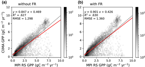
In our global simulations, annual mean GPP may increase by >0.7 μmol m−2 s−1 in a grid (Figure 8a), corresponding to >7% changes in GPP (relative to the GPP without UV/FR improvements; Figure 8c). ΔGPP was highest in the tropical rainforests, followed by the temperate and boreal forests; and ΔGPP was minimal in the arid regions (Figure 8). Given the seasonal changes in LAI, CHL, CI, and RAD, ΔGPP also showed seasonality, particularly in the middle- and high-latitude regions (Figure S7). For example, ΔGPP was highest in the summer in the north hemispherical temperate and boreal forests whereas showed little seasonality in the tropical rainforests or arid regions (Figure S7). Integrated globally, we got a GPP of 127.3 PgC year−1 compared to 122.6 PgC year−1, respectively, namely a 4.6 PgC year−1 difference in GPP (3.8% increase). The spatial patterns of GPP with UV + FR implementations agreed with the MPI RS GPP slightly better than that without UV + FR implementations: the slope of linear regression was closer to 1, R2 of linear regression was a bit higher, though RMSE was slightly higher (Figure 9).
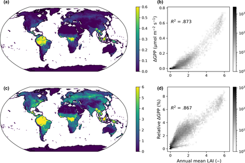
When correlating ΔGPP to annual mean LAI, we found that the spatial patterns of LAI best explained the spatial patterns of ΔGPP (R2 = .873; Figure 8b). In comparison, the R2 was .259 and .233 for CHL and CI, respectively. Regarding the relative change in annual mean GPP per grid, LAI alone explained 86.7% of the variation (namely R2 = .867), whereas CHL and CI explained 15.4% and 28.7%, respectively. Our simulation results highlight the necessity to improve FR and photosynthesis representations in LSMs, particularly in regions with high LAI.
The PAR albedo showed high spatial variations globally, being highest in the barren and boreal regions and lowest in the tropical and temperate forests (Figure 10a). In comparison, the UV albedo showed lower spatial variations in vegetated areas given the lower UV albedo values (Figure 10b). Because of the higher UV absorption by plants, using PAR albedo to proxy UV albedo would result in overestimated surface albedo, showing the lowest bias in the tropical regions (<0.01) but the highest bias in the high latitude areas of the north hemisphere (>0.1; Figure 10c). The majority of the vegetated regions had a bias >0.02 (Figure 10c; see Figure S8 for the same maps with an upper bound of 0.02).
4 DISCUSSION
Incorporating UV explicitly into canopy RT would result in a more accurate surface energy budget, particularly in the vegetated regions. If assuming an average of 0.03 UV albedo bias, it is equivalent to a global mean of ≈1.4 W m−2 overestimation of the surface reflected UV, and the bias would potentially propagate and lead to divergent climate projections. Nevertheless, it requires more investigation using coupled ESMs to understand how the biased surface energy budget would impact climate modeling. While the UV representation improves the energy budget, the damages of UV (particularly the shorter wavelength UV) to the photosystems are not accounted for in our model (neither in other LSMs). For example, Brandle et al. (1977) reported that leaf photosynthetic rate continuously decreased with short-term UV exposure for a few hours; Strid et al. (1990) found that leaf pigments (such as chlorophyll and carotenoid) and the photosynthetic rate decreased with time after long-term UV exposure for a few days; Nogués et al. (1998) found lower photosynthetic rate and stomatal conductance for plants grown under supplemental UV; and Poulson et al. (2006) found elevated stomatal conductance for drought-stressed plants grown under supplemental UV. Thus, simply counting UV contribution to the energy budget and PPAR without addressing the damages to the photosynthesis system could probably result in an overestimated assimilation rate and an underestimated stomatal conductance during drought. However, the current understanding of UV's impact on photosystems is not adequate to be quantitatively represented in photosynthesis models, and further investigations of the dynamics of photosystem damage and repair will help resolve the problem.
Per the FR implementation, although our simple correction over PPAR helps explain the observed photosynthetic rates in responses to various light sources, a more detailed representation of the photon partitioning between PSI and PSII would help more accurately model the vegetation processes. For example, a per wavelength photon partitioning function as suggested in Laisk et al. (2014) could be used to compute PPAR for each photosystem, and then computing the effective PPAR using Equation (7) could be more accurate. However, whether the photon partitioning scheme reported in Laisk et al. (2014) is generally applicable to other leaves or species with various leaf pigments needs to be further investigated. Moreover, it is also possible that photosynthesis is limited by ATP production rather than NADPH production when computing the light-limited photosynthetic rate (Farquhar et al., 1980; Yin et al., 2021). In this case, PSI's extra FR photon absorption stimulates ATP production, even if the UV + PAR photon partitioning between PSI and PSII does not change. Explicitly modeling the state transition and supplies of ATP and NADPH in the electron transport pathway would help better model photosynthesis. Further, the photon partitioning between PSI and PSII could also impact the computation of solar-induced chlorophyll fluorescence (SIF) because PSI and PSII have different SIF emission spectra. As a result, the effective SIF quantum yield and spectrum should be weighted based on the actual photon partitioning. However, the fluorescence models that compute PSII quantum yield only (Han et al., 2022; van der Tol et al., 2014) are not capable of making corrections based on photon partitioning. Comparatively, the Johnson and Berry (2021) model computes the SIF quantum yields for both PSI and PSII, hence being potentially useful to advance SIF modeling in canopy RT schemes. Yet, the model remains to be tested intensively with data before being applied to large-scale simulations.
Given the importance of UV and FR in photosynthesis and surface energy budget, it is crucial for LSMs to account for the two explicitly in their RT schemes, e.g., through adding more bands in parallel to PAR and NIR. However, extending the PPAR definition in traditional broadband RT models is challenging because the broadband RT models are not capable of accounting for the action spectra of chlorophyll or light source spectra. As a result, even the PAR and photosynthesis profile within the vertical canopy are subject to biases caused by radiation spectra (Figure 2) and leaf traits such as CHL (Wang & Frankenberg, 2024). For instance, if the FR band is separated from NIR and the PAR absorption coefficient is used for the FR band, the modeled PPAR would be overestimated. If the NIR absorption coefficient is used for the new FR band, the modeled PPAR would be underestimated. In reality, the fraction of FR photons in PPAR in total radiation would (1) differ between sunlit and shaded leaves and (2) vary with canopy depth. Therefore, though being more computationally expensive, implementing a hyperspectral RT scheme into LSMs would help resolve these problems. At least, before the LSMs are fully moved to hyperspectral, empirical corrections should be made to account for the variations in vegetation parameters caused by radiation spectra and plant traits (see Wang and Frankenberg (2024) for an example of improving the electron transport parameterization in broadband RT models).
Estimation of terrestrial land carbon fluxes largely relies on interpolating flux towers measurements (e.g., Jung et al., 2017; Tramontana et al., 2016), correlating remote sensing data (e.g., Running et al., 2021; Zhang et al., 2017), and making global-scale LSM simulations (e.g., Lawrence et al., 2019; Melton et al., 2020) (see Zhang & Ye, 2021 for an overview of 45 GPP products). However, given the different models and major drivers, there is no consensus on global GPP, and the GPP products predict a globally integrated GPP range from 80 to 180 PgC per year (Jung et al., 2020). As there is no golden standard for GPP, it cannot be determined whether including UV and FR's contribution to photosynthesis improves the GPP estimation. Further, one can easily optimize the model parameters and weather drivers to align site-level predictions with observations, thus improving the modeled GPP. Yet, we should distinguish “improvements” in model parameterization (such as model formulations and processes) and parameters (such as formulation constants and plant traits). The parameterization is meant to make the modeled result more reasonable, such as the use of stomatal models to represent plants' responses to environmental cues (Ball et al., 1987; Medlyn et al., 2011; Sperry et al., 2017) and the UV and FR implementations in the present study; the parameters are meant to feed the parameterization schemes and make them more pragmatic, such as the use of leaf reflectance and transmittance look-up table in LSMs and the global CHL dataset used to derive leaf reflectance and transmittance (Croft et al., 2020). Therefore, implementing the new UV and FR representations in other LSMs and statistical models, such as the light-use efficiency GPP models (Running et al., 2021; Zhang et al., 2017), could make the models more reasonable; further optimization of the model parameters would improve the models' predictive skills.
Running canopy RT at hyperspectral mode would further allow simultaneously simulating canopy optical properties, including canopy reflection and fluorescence, which are often used in remotely sensing vegetation processes. Particularly, the UV implementation into the hyperspectral RT also enables learning from remote sensing data in the UV band. For example, the shortwave spectrum of Earth Surface Mineral Dust Source Investigation (EMIT) extends to 380 nm (Green et al., 2020); Global Ozone Monitoring Experiment 2 (GOME-2) has two channels covering 240–315 nm and 311–403 nm (Munro et al., 2016); Greenhouse gases Observing Satellite (GOSAT) has a UV band covering 370–390 nm (Nakajima et al., 2012); and TROPOspheric Monitoring Instrument (TROPOMI) has two channels on 300–320 nm and 320–405 nm (Veefkind et al., 2012). These satellite platforms would provide valuable data for calibrating the land surface processes.
5 CONCLUSIONS
UV plays an important role in surface energy balance but has been neglected or treated equally as PAR in vegetation and LSMs, potentially resulting in biased energy budgets and photosynthesis modeling. FR, on the other hand, has been accounted for as NIR in the surface energy budget, but its enhancement to photosynthesis due to chlorophyll absorption has not been accounted for in any of the photosynthesis models. We explored how the improved representation of UV and FR may change the canopy RT and photosynthesis modeling at the site and global scales using a next-generation LSM—CliMA Land. We found that after accounting for UV in CliMA Land, the model predicted increased net absorbed energy and hence canopy temperature; however, the modeled photosynthetic rate showed marginal change. With the improved FR representation in the canopy RT and photosynthesis modeling, we found increased GPP and transpiration rates. The changes in GPP respond to CHL, LAI, CI, and RAD. At the global scale, GPP in a grid might increase by >7% in the tropics that have the highest LAI whereas the globally integrated GPP increased by 3.8%. The surface UV albedo may be biased by more than 0.1 if proxied by PAR albedo. Our findings highlight the necessity of improving UV and FR representations in LSMs and ESMs.
AUTHOR CONTRIBUTIONS
Yujie Wang: Conceptualization; data curation; formal analysis; investigation; methodology; resources; software; validation; visualization; writing – original draft; writing – review and editing. Renato K. Braghiere: Formal analysis; methodology; visualization; writing – review and editing. Yi Yin: Investigation; visualization; writing – review and editing. Yitong Yao: Investigation; visualization; writing – review and editing. Dalei Hao: Investigation; visualization; writing – review and editing. Christian Frankenberg: Conceptualization; funding acquisition; investigation; methodology; supervision; visualization; writing – review and editing.
ACKNOWLEDGEMENTS
This research has been supported by the National Aeronautics and Space Administration (NASA) Carbon Cycle Science grant 80NSSC21K1712 and OCO2/3 Science Team 80NSSC21K1075 awarded to CF. CF acknowledges support from Schmidt Sciences, LLC. This research was partially carried out at the Jet Propulsion Laboratory, California Institute of Technology, under a contract with the National Aeronautics and Space Administration. This material is based on the MOFLUX site supported by the U.S. Department of Energy, Office of Science, Office of Biological and Environmental Research Program, Climate and Environmental Sciences Division through Oak Ridge National Laboratory's Terrestrial Ecosystem Science Scientific Focus Area. We appreciate the constructive suggestions provided by the anonymous reviewers. California Institute of Technology. Government sponsorship acknowledged (Copyright 2024. All rights reserved).
CONFLICT OF INTEREST STATEMENT
The authors declare no conflict of interest.
Open Research
DATA AVAILABILITY STATEMENT
The version of CliMA Land used to run global simulations (simulation tag “a12”) is openly available in Zenodo at https://doi.org/10.5281/zenodo.10652942 (CliMA Land Team, 2024a). The data that support the findings of this study are available in Zenodo at https://doi.org/10.5281/zenodo.10652972 (CliMA Land Team, 2024b). Global datasets used to feed to CliMA Land and perform the analysis can be accessed at https://data.caltech.edu/records/mwhhr-0rq03 and https://doi.org/10.5281/zenodo.8345558 or by using GriddingMachine (https://github.com/CliMA/GriddingMachine.jl).


