The case for increasing the statistical power of eddy covariance ecosystem studies: why, where and how?
Abstract
Eddy covariance (EC) continues to provide invaluable insights into the dynamics of Earth's surface processes. However, despite its many strengths, spatial replication of EC at the ecosystem scale is rare. High equipment costs are likely to be partially responsible. This contributes to the low sampling, and even lower replication, of ecoregions in Africa, Oceania (excluding Australia) and South America. The level of replication matters as it directly affects statistical power. While the ergodicity of turbulence and temporal replication allow an EC tower to provide statistically robust flux estimates for its footprint, these principles do not extend to larger ecosystem scales. Despite the challenge of spatially replicating EC, it is clearly of interest to be able to use EC to provide statistically robust flux estimates for larger areas. We ask: How much spatial replication of EC is required for statistical confidence in our flux estimates of an ecosystem? We provide the reader with tools to estimate the number of EC towers needed to achieve a given statistical power. We show that for a typical ecosystem, around four EC towers are needed to have 95% statistical confidence that the annual flux of an ecosystem is nonzero. Furthermore, if the true flux is small relative to instrument noise and spatial variability, the number of towers needed can rise dramatically. We discuss approaches for improving statistical power and describe one solution: an inexpensive EC system that could help by making spatial replication more affordable. However, we note that diverting limited resources from other key measurements in order to allow spatial replication may not be optimal, and a balance needs to be struck. While individual EC towers are well suited to providing fluxes from the flux footprint, we emphasize that spatial replication is essential for statistically robust fluxes if a wider ecosystem is being studied.
Introduction
The eddy covariance (EC) technique provides one of the most direct measures of energy and mass exchanges between the land surface and the atmosphere (Baldocchi, 2008, 2014). A major strength of EC is its unique ability to provide a time series of spatially integrated flux estimates at the footprint scale. In recent decades, EC has become the de facto approach for estimating land–atmosphere fluxes of terrestrial ecosystems. Collaboration between researchers has resulted in global networks (Baldocchi et al., 2001; Baldocchi, 2008, 2014), and these have provided numerous invaluable advances in our understanding of – for example – ecosystem dynamics (Lasslop et al., 2010; Migliavacca et al., 2011; Raczka et al., 2013; Stoy et al., 2013). Notwithstanding these valuable contributions, we contest that the statistical power of EC studies could be improved if the current lack of spatial replication was addressed.
It is perhaps useful at this early stage to consider replication in the context of EC studies. If for a moment, we consider a typical scenario: an EC tower sited in a field containing a common crop. For the sake of argument, let us assume that the field is uniformly managed, perfectly flat and extends over a much larger area than the flux footprint; that is, it is ideally suited to EC. This scenario presents at least three distinct units for which a researcher may wish to report fluxes: (i) the footprint, (ii) the field, and (iii) the wider ecosystem. In this example, the specification of the ‘ecosystem’ would include surrounding areas with the same crop type and environmental conditions, and would likely be much larger than either the footprint or field. In reporting a flux for any of these units, researchers must account for measurement error; however, it is only for the two larger units that spatial replication is needed. Notwithstanding the time-varying nature of the footprint (Vesala et al., 2008), ergodicity and the temporal replication of EC allow researchers to provide statistically robust flux measurement for the footprint using a single tower (Hollinger et al., 2004; Schmidt et al., 2012). In contrast, EC studies reporting fluxes for the field, or wider ecosystem, must use independent spatial replicates to account for any spatial variability in the flux (Hurlbert, 1984, 2004). The use of a single EC tower to report a flux for a region that extends beyond the measurement area, that is the flux footprint, would be to risk statistical misrepresentation through temporal pseudoreplication (Hurlbert, 1984). Such an approach contains the implicit assumption that the spatial variability – and thus the sampling variability – is negligible. A look at the literature will reveal that this assumption is common and individual EC systems are routinely employed to represent the ecosystem in which they are situated, and not just their flux footprint, as noted by Oren et al. (2006).
Theoretically, the uncertainty associated with EC sampling variability could be eliminated if a flat, spatially homogenous surface (including fluxes), with atmospheric and environmental conditions that exhibit stationarity, can be found (Hurlbert, 1984). However, EC studies rarely – if ever –satisfy these basic theoretical assumptions (Finnigan et al., 2003; Aubinet & Feigenwinter, 2010), and it is even rarer for studies to empirically demonstrate spatial homogeneity of fluxes (Peltola et al., 2015).
Assumptions of flux homogeneity tend to rely on a qualitative and/or quantitative assessment of the spatial variability in some visible properties of the vegetation. However, this assumption ignores many difficult to measure factors known to vary spatially and influence C fluxes (Peukert et al., 2013; Glendell et al., 2014; Mbufong et al., 2014). It also ignores the evidence from both chamber and EC studies which have observed intra-ecosystem spatial variability of fluxes (Katul et al., 1999; Bubier et al., 2003; Oren et al., 2006; Riveros-Iregui & McGlynn, 2009; Peltola et al., 2015).
The role of spatial variability at many sites and/or ecosystems is largely unknown as such a small proportion of studies undertake spatial replication; however, one study demonstrated that, for an apparently uniform pine plantation, spatial variability can contribute ~50% of the total uncertainty in annual net ecosystem exchange (NEE; Oren et al., 2006). Thus, in addition to any measurement error, the uncertainty due to spatial sampling variability must also be included in the total uncertainty on the flux from an ecosystem (Smith, 2009; Davis et al., 2010; Post et al., 2015).
- Why is spatial replication rare in EC studies?
- Where is the lack of spatial replication most acute?
- How much spatial replication is required to be statistically rigorous?
- How can we improve the statistical power of EC studies?
- Could inexpensive, albeit, less accurate EC systems improve statistical power?
We then describe an inexpensive EC system that can, in some circumstances, provide a cost-effective solution to improving the statistical power of EC studies. Finally, we consider some issues and risks involved in seeking to improve spatial replication and statistical power.
Why is spatial replication rare in EC studies?
EC measurements are rarely replicated: of the 130 studies published in 2015 using CO2 EC data – search via the Web of Knowledge (http://wok.mimas.ac.uk/), terms ‘eddy covariance AND carbon dioxide’ – 21% were based on data from ad hoc networks such as FLUXNET, 27% of studies used at least two towers (though not necessarily on the same surface type) and 52% used just one EC tower. Only 3% of studies initiated intrasite EC replication of a surface type.
It is instructive to consider the factors contributing to the continuing lack of spatially replicated EC: Firstly, the theoretical basis for EC was laid down in the early 20th century, decades before the first EC carbon dioxide flux measurements in the 1970s (Desjardins, 1974; Baldocchi, 2003). EC remained at the cutting edge of what is technologically and logistically feasible for many decades (Desjardins & Lemon, 1974; Bingham, 1978; Ohtaki & Matsui, 1982), and it was not until 1990 when the first annual study commenced (Wofsy et al., 1993). Secondly, EC developed from the fields of fluid dynamics and micrometeorology where the focus is more on the nature of atmospheric structures: the variability of ecosystem processes being of secondary import.
- Inertia: Many fields of science are slow to improve on well-established protocols (Collins, 1985). The recent debate surrounding the (mis-)use of P-values provides an example of the inertia that can perpetuate certain methods despite improvements being demonstrated (Nuzzo, 2014).
- Effort: EC requires a considerable logistical effort. This effort is multiplied when the ecosystem is remote, in a hostile environment, has a tall canopy or involves challenging data analysis. However, as evidenced by the existing studies, if the benefits are perceived to be sufficient, researchers can (and will) undertake logistically complex projects. Thus, particularly in ecosystems amenable to EC, effort may not be the factor limiting spatial replication.
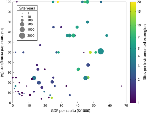
- Cost: EC equipment is expensive, and cost can be a factor limiting the spatial replication of EC (Gong et al., 2015; Post et al., 2015). The gross domestic product (GDP) of a country correlates with the site years of EC data that country produces (Fig. 1). The very fact that very few published EC studies use replication may act as an impediment to any researcher seeking additional funds to adequately replicate EC. Researchers may struggle to find the precedents in the peer-reviewed literature illustrating the need to spatially replicate EC.
Where is the lack of spatial replication most acute?
Schimel et al. (2015) highlights the mismatch between the global distribution of EC towers and the latitudinal peak in land surface productivity in the tropics. These results are confirmed when we consider how the network of EC towers samples the Earth's >800 ecoregions (Olson et al., 2001). Despite the classification of ecoregions remaining a very broad, globally only 23% are sampled by EC measurements (Table 1). The ecoregions are particularly poorly sampled in some regions: Africa 9%, Oceania (excluding Australia) 5% and South America 12%. At the country level, wealthy countries, with a higher per capita gross domestic product (GDP), are able to sample a higher proportion of their ecoregions and do so with more replication (Fig. 1).
| Continent | Ecoregions (#) | Site years (#) | Sampled (#) | Sampled (%) |
|---|---|---|---|---|
| Africa | 126 | 151 | 11 | 9 |
| Asia | 276 | 1208 | 53 | 19 |
| Australia | 40 | 208 | 15 | 38 |
| Europe | 54 | 2033 | 30 | 56 |
| North America | 190 | 2627 | 68 | 36 |
| Oceaniaa | 38 | 26 | 2 | 5 |
| South America | 118 | 342 | 14 | 12 |
| Antarctica | 7 | 0 | 1 | 14 |
| Total | 849 | 6595 | 194 | n/a |
- a Oceania excluding Australia.
How much spatial replication is required to be statistically rigorous?
The relationship between statistical power, replication and effect size
When comparing fluxes from different ecosystems, statistical power provides a useful metric of our ability to measure differences. Statistical power is the probability of correctly rejecting a null hypothesis; for example H0, there is no difference in the fluxes from the two ecosystems. Aiming for a statistical power ≥0.95 implies we are willing to accept a 5% chance of a type II error, that is we will not measure a difference when, in fact, a difference exists.
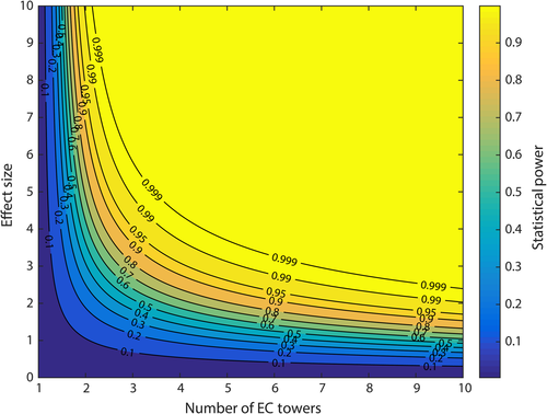
Statistical power is a function of the number of independent replicates and the effect size (Fig. 2). Effect size is the magnitude of the difference in mean fluxes from two ecosystems, relative to the total measurement uncertainty (Eqn 1). A large effect size implies a relatively large difference in the mean fluxes compared to a relatively small total uncertainty; that is, differences should be readily observable. For large effect sizes, comparatively few systems are needed: above an effect size of six, just two independent replicates per surface are adequate to achieve a statistical power of 0.95. More towers are needed as the effect size drops, and for a moderate effect size of three, at least four replicates are required. By the time the effect size drops to ≤1.7, the number of replicates has risen to be >10. Thus, researchers should pay careful attention to the minimum expected effect size as a key parameter when planning EC studies.
Estimating effect size
 (1)
(1) is the mean flux from ecosystem 1,
  is the mean flux from ecosystem 2 and
  is the pooled standard deviation for the total uncertainty from both ecosystems (Eqn 2). The total uncertainty for an ecosystem combines both the measurement uncertainty and the uncertainty due to sampling variability.
 (2)
(2) is the sample size for ecosystem 1,
  is the sample size for ecosystem 2,
  is the standard deviation of the total uncertainty from ecosystem 1 and
  is the standard deviation of the total uncertainty from ecosystem 2.
 (3)
(3) is the mean flux for the ecosystem,
  is the standard deviation for the total uncertainty from the ecosystem and F is the comparison flux value.
Typical effect sizes for EC studies
Due to the lack of replicated EC studies, the sampling variability for most ecosystems remains unknown. From Eqns 1-3, it is clear that without estimates of sampling variability, we cannot calculate the effect size. However, we can estimate a best case (i.e. maximum effect size) based just on measurement error, that is under the assumption that spatial sampling variability is zero. For example, let us consider the case where we are trying to determine whether the mean annual flux from a typical ecosystem is significantly different from zero. We shall take our mean measured flux,  , to be the mean annual uptake for the FLUXNET sites, that is 156 gC m−2 yr−1 (Baldocchi, 2014). Assuming the site is ideally suited to EC, the measurement error is approximately ±50 gC m−2 yr−1 (Baldocchi, 2003). Therefore, using Eqn 3, we calculate the effect size, d = 3.1. Alternatively, for a nonideal site, our annual measurement error increases to around ±200 gC m−2 yr−1, and d drops to 0.78.
How many towers are needed?
The commonly used formulae for estimating sample sizes are not suitable for sample sizes below 30. Instead, under the assumption of a normal distribution in the fluxes, an iterative algorithm based on T-scores should be used. In lieu of a simple equation, Fig. 3 can be used to estimate the minimum required number of towers (generated using the sampsizepwr function from matlab R2015b). We set the significance value to be 1 minus the statistical power, that is if the statistical power is 0.95, the significance value will be 0.05. To determine the number of towers required, you should follow these steps:
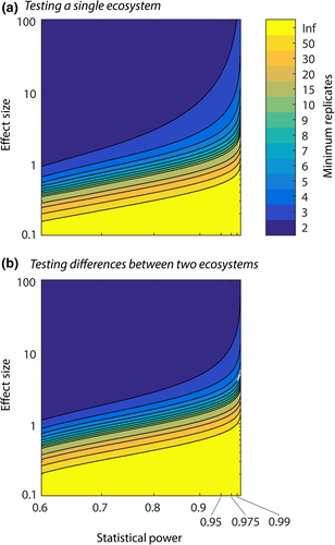
Step 1: Determine the appropriate reference panel of Fig. 3. If you wish to test whether the flux from a given surface is significantly different from zero, then use Fig. 3 Panel a, otherwise, if you are contrasting fluxes from two ecosystems, use Fig. 3 Panel b.
Step 2: Estimate your minimum expected effect size using Eqns 1 or 3, as appropriate.
Step 3: Decide on an appropriate statistical power. A value of 0.95 is often used in ecological studies, although it should be noted that this value is somewhat arbitrary.
At a typical ideal site – with an effect size of 3.1 – we need at least four EC replicates to achieve our chosen statistical power of 0.95. If the site were nonideal – with an effect size of 0.78 – then the same four towers would only give us a statistical power of ~0.2. That is, 80% of the time we would fail to detect the genuinely nonzero flux. To have 95% confidence that our nonideal site is a sink, we would need 24 towers. Finally, we note that chamber flux studies have indicated that the magnitude of fluxes may not be normally distributed (Riveros-Iregui & McGlynn, 2009). In this situation, nonparametric statistics will be required.
How can we improve the statistical power of EC studies?
We can improve the statistical power by either increasing the effect size or increasing the replication used in the study (Fig. 2).
Increasing effect size
It would be illogical to prioritize effect size – and thus site selection – at the expense of the scientific and/or societal import of a research question. Therefore, to maximize effect size, we must consider how we analyse the data. While the diversity of ecosystem responses precludes a universal approach to maximizing effect size, identifying effects in processes with simpler dependencies is more likely to be successful. For example, at an old growth forest site with a near-neutral carbon balance, considering gross fluxes (i.e. GPP, respiration) may be more successful than considering NEE.
Increasing spatial replication
At least two EC towers are required to have any statistical power for areas larger than the flux footprint. The number of independent spatial replicates required increases for effect sizes below six. To increase spatial replication, we could broaden definitions of our ecosystem to encompass more existing EC systems or use more EC systems to sample the ecosystem. An analysis of current EC sampling of ecoregions (Table 1 and Fig. 1) demonstrates that even these very broad categories result in poor replication for many ecosystems. Therefore, while it might be appropriate to broaden definitions for certain studies, the loss in specificity in an ecosystem's definition is likely to erode our ability to address scientifically and socially meaningful questions. Additionally, if the resulting fluxes have greater flux variability, the overall result may actually decrease effect size.
Therefore, to improve replication in a specific ecosystem, we must either (i) relocate existing towers, (ii) increase investment, or (iii) reduce the cost of deploying EC. Relocating existing EC systems will improve replication for a few ecosystems at the expense of eliminating measurements in many other ecosystems. Increased financial support for widespread EC replication only seems likely if the underlying problem can be more clearly demonstrated to be critical to societal well-being.
An alternative approach is to ignore categorical classifications (i.e. discrete ecosystems) and instead use a numerical quantification of each site's characteristics on a gradient (e.g. Emanuel et al., 2006; Stoy et al., 2006; Baldocchi, 2008). Using this approach, statistically significant correlations between fluxes and quantifiable site properties can be found (Baldocchi, 2008; Whelan et al., 2015). Only certain research questions are amenable to this type of experimental design, and it does not allow researchers to test whether a particular ecosystem is a carbon sink, nor can it indicate whether the fluxes from two ecosystems are different from each other.
Could inexpensive, less accurate EC systems improve statistical power?
When cost is not an issue, it will always be preferable to have the most accurate EC system possible. It is, however, likely that most researchers would welcome a system that only cost 5% of a conventional system, if it maintained 95% of the accuracy. However, these same researchers are unlikely to be enthusiastic about a system that delivers 5% of the accuracy, but still costs 95% of the traditional system. In this section, we quantify these cost-accuracy trade-offs with the aim of maximizing statistical power for a given amount of funding.
As the absolute error of an EC system depends on many factors, we employ a normalized measurement uncertainty when comparing the trade-off between accuracy and cost of a nominal EC system. As a reference, standard errors of the mean from this hypothetical conventional tower are normalized to have a value of ‘1’ (Fig. 4). We could match this accuracy using measurements from two EC towers which have uncertainties 40% higher or four EC towers that have uncertainties 100% higher (Fig. 4). The number of EC systems we can afford is inversely related to the cost of each EC system: the less accurate systems would need to cost <50% and 25% of a conventional EC system, respectively. Fixed costs, such as towers, data storage and personnel time will become increasingly more significant for lower cost systems, although some savings will be obtained through economies of scale for these costs. However, as these costs are variable, they cannot be included in a meaningful comparison.
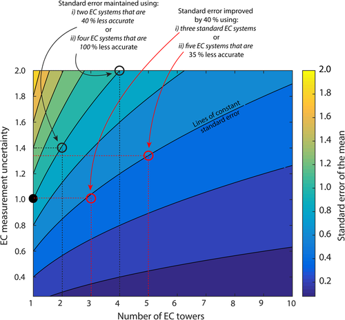
As a second example, we may wish to improve the overall standard error by 40%; this can be achieved by replacing a single conventional EC system with three conventional systems or five systems with 35% higher uncertainty (Fig. 4). In this case, the less accurate systems would have to be <60% of the cost of a conventional system to make economic sense.
If we again consider the typical Fluxnet site (i.e. 156 ± 50 gC m−2 yr−1), we showed that we needed four standard towers to have 95% confidence that this flux was nonzero. If we used EC systems with 50% more noise (i.e. 156 ± 75 gC m−2 yr−1), we would need six EC systems, and the cost of these systems should be ≤67% of a normal EC system to be economical.
Cost and accuracy requirements
The preceding analysis indicates that the trade-off between cost and accuracy is complex, but that an inexpensive system would be useful in a number of situations if it were around ≤67% of the cost, while having an increase in measurement error of ≤50%. Compared to commonly used EC instrumentation, off-the-shelf alternatives exist that can deliver these cost saving for the anemometer and datalogger, with a minimal increase in errors. Therefore, we focus on the most expensive component of the system, for which an off-the-shelf solution does not currently exist: the CO2 and H2O infrared gas analyser (IRGA).
Inexpensive CO2 and H2O sensors
The inexpensive CO2 and H2O sensor for our EC system is based on a Vaisala GMP343 CO2 sensor (hereafter referred to as the GMP343) and a Honeywell HIH-4000 relative humidity (RH) sensor (hereafter referred to as the HIH-4000). The GMP343 IRGA is environmentally sealed to IP67 levels and uses <1 W of power. We used the 0–2000 ppm diffusion IRGA which had a quoted accuracy of ±5 ppm +2% of the reading and a frequency response equivalence of 0.74 Hz. The GMP343 costs an order of magnitude less than the current state-of-the-art CO2 EC sensor. For water vapour measurements, we employ an HIH-4000 capacitive sensing chip with an accuracy of ±3.5% relative humidity, a typical response time of 5-s in slow-moving air and a power draw of ~1 mW. The sensor costs <£20 and is resistant to wetting, dust and oils.
Inexpensive EC system configuration
Two inexpensive systems are tested: one with just a GMP343 (system #1) and a second with a GMP343 and a HIH-4000 (system #2). For each system, the sensors are housed in an aluminium enclosure to improve wet-weather performance and reduce the effects of temperature fluctuations (Clement et al., 2009). The enclosure is flushed by an axial fan every ~0.1 s. Further details of the sensors are available in Appendix S1 and the enclosure in Appendix S2.
A LI-COR LI-7500 (hereafter referred to as the LI-7500) provides the corroborating flux measurements. The LI-7500 is placed in an enclosure with an internal volume (excluding the sensor) of 0.4 litres, which is flushed every 0.1 s by an axial fan (Clement et al., 2009). The inexpensive sensors and the LI-7500 share the same Campbell Scientific CSAT3 anemometer and are all recorded by a Campbell Scientific CR5000 datalogger. Details of the LI-7500 setup are provided in Appendix S3.
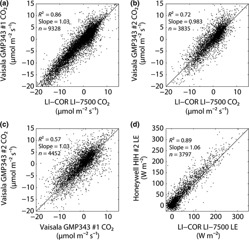
Fluxes were calculated for 30-min periods using edire (version 1.5.0.50). The overall correction applied was the following: 18% for the LI-7500 CO2 flux, 42% for the LI-7500 LE flux, 52–55% for the GMP343 CO2 flux and 133% for the HIH-4000 LE flux (Fig. 5). Full details of this processing routine are given in Appendix S4, with the frequency response corrections described in Appendix S5 and the cospectral model in Appendix S6.
Corroborating the inexpensive EC fluxes
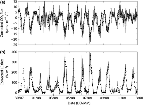
Corrected fluxes for the low-cost systems show good agreement with the LI-7500 control. The two GMP343 systems have regression slopes of 1.03 and 0.98 (Fig. 5), that is a disagreement in the overall CO2 flux magnitude of between 2% and 3%. There is strong agreement between the GMP343- and LI-7500-based fluxes, with the coefficient of determination, R2, ranging from 0.72 to 0.86. The lower R2 for the second system is attributed to the lower autumn fluxes when this system was added. The slope of the Honeywell HIH-4000 and the LI-7500 is 1.06, equating to a 6% bias in the flux magnitude. The HIH-4000 and LI-7500 LE fluxes have a R2 of 0.89. Strong visual agreement between conventional and low-cost fluxes is evident in time series plots (Fig. 6).
The magnitude of flux loss, and therefore the applied frequency correction, increases significantly with stability and wind speed (Fig. S7). We therefore expect any biases in flux frequency corrections for the low-cost EC system to become larger at high wind speeds: we do not find evidence of wind speed dependence on the median residuals between the LI-7500 and low-cost system's fluxes (Fig. S8). The corrected fluxes from the low-cost system are free from bias even with large frequency correction factors. Instead, when high wind speeds necessitate larger frequency corrections, the spread of the residual flux quantiles increases, confirming expectations that large correction factors amplify the noise inherent in the raw fluxes.
The measurement error of the inexpensive system
The uncertainty of the flux measurements is assessed using a self-referential approach that is performed separately for each system (Hollinger & Richardson, 2005). These estimates of random errors suggest that the low-cost system has 37% higher uncertainty for CO2 fluxes and 20% higher uncertainty for LE fluxes. See Appendix S9 for further details.
The relative cost of the inexpensive system
Our custom GMP343 and HIH-4000 enclosures cost between ~15% and 25% of a conventional CO2 and H2O IRGA. Therefore, for many situations where statistical power needs improvement, the reduced accuracy of the inexpensive system is more than offset by the higher replication afforded by the cost savings.
A trial deployment of seven EC systems
In a further trial of the inexpensive system, three inexpensive (GMP343/HIH-4000) systems were installed alongside four conventional systems in an agricultural field near Dumfries, United Kingdom. The inexpensive systems were installed at 4.5 m. The conventional systems included a closed path LI-COR LI-7000 (at 11 m), two enclosed LI-7500 systems (at 4.5 m) and a Campbell Scientific IRGASON (at 2.5 m). The inexpensive and conventional systems provided qualitatively similar performance (Fig. 7).
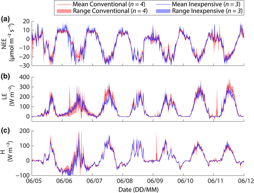
The Hollinger uncertainty estimates suggest that the mean MAD (mean absolute deviation) for CO2 was 3.7 for the conventional systems (excluding the IRGASON, which due to poor wet-weather performance had a MAD of 5.2) and 4.9 for the inexpensive systems (See Appendix S10 for details). For the LE, the mean MAD was 7.4 for the conventional systems (excluding the IRGASON, which due to poor wet-weather performance had a MAD of 26) and 7.7 for the inexpensive systems. For this deployment, the inexpensive systems had random uncertainties that were ~32% higher for CO2 and ~4% higher for LE, relative to the conventional systems (again excluding the IRGASON). These MAD values indicate we are well within the ≤ 67% accuracy requirement for inexpensive systems to be useful.
The colocation of multiple EC systems in this manner means we do not need to rely on the Hollinger approach to estimate random errors; instead, we can pair EC systems and calculate the differences for every half-hourly period. While the MADs remain similar for CO2, the MADs for LE increase by 126% for the conventional systems and 155% for the inexpensive systems. It can be shown that this increase is due to the filtering applied as part of the Hollinger approach. Therefore, at our site, the Hollinger approach dramatically underestimates the actual random error of LE measurements.
Other considerations
Which came first: the chicken or the egg?
In this study, our metaphorical ‘chickens’ and ‘eggs’ are replaced with ‘spatial replicates’ and ‘uncertainties’. Without independent spatial replication, we cannot estimate the sampling variability for an ecosystem and thus total uncertainty. Without total uncertainty, we cannot estimate effect size. Finally, without effect size, we cannot accurately estimate the number of replicates we need. Therefore, until more studies have independently replicated EC measurements, indicative effect sizes are unknown and it would be prudent to use the minimum likely effect size.
Nonreplicated EC studies are still vital
This study considers the specific case of contrasting different ecosystems: the conclusions of this study are not intended to relate to studies considering fluxes from specific EC footprints. Many research questions focus on temporal changes, drivers and processes and do not attempt to apply results to a wider domain and thus do not require spatial replication. Watershed-scale hydrological studies, for example, provide a clear example of valuable experimental designs that have limited spatial replication (Ice & Stednick, 2004; Nippgen et al., 2016). Also, certain ecosystems (e.g. a small field) may be too small to be replicated with EC. Therefore, we emphasize that not all EC studies would necessarily benefit from replication. Similarly, funding constraints may mean an ecosystem could be measured with very limited replication, or not measured at all. Even if the replication needed for high statistical power across the wider ecosystem cannot be achieved, the information gained from the flux footprint time series can be invaluable.
The risks associated with improving statistical power
There is a risk that a focus on improving statistical power using greater independent spatial replication may have unintended negative consequences. The additional effort required for replication may mean that important ecosystem, or ancillary data, may be neglected. Furthermore, inexpensive EC system we describe requires larger frequency corrections, and consequently, greater care must be taken in the processing of fluxes to avoid large systematic biases. It is likely that a minimum deployment period may be required to allow proper characterization of the site's turbulent characteristics, thus making low-cost systems less attractive for very short-term deployments. Until these inexpensive systems have been widely tested, we recommend that at least one conventional system be available for direct comparison.
Conclusions
Only 3% of the EC studies of CO2 fluxes published in 2015 incorporated ecosystem replication into their experimental design. Over half the studies published in 2015 relied on a single EC system and therefore lack the statistical power to extend their findings beyond their flux footprint. These studies are still invaluable, but researchers need to pay close attention to how results are presented. For example, a single tower located in a managed forest plantation cannot provide a statistically robust answer to the question: What is the carbon sequestration potential of this managed forest plantation? Instead, the single tower can address the question: What is the carbon flux of the managed forest plantation in the flux footprint?
When the goal of an EC study is to compare ecosystems, or demonstrate a particular ecosystem to be a sink or source, we argue that multiple towers are needed. For these purposes, a minimum of two EC towers are required, but for low effect sizes, this number can be far higher. Due to a lack of replicated EC studies, typical effect sizes for different ecosystems are not well known, and so, we recommend researchers use a conservative estimate of effect size when determining the level of spatial replication needed.
We describe and test an inexpensive EC analyser for CO2 and H2O fluxes that can help improve spatial replication and thus statistical power. Finally, while greater replication is needed, there are also risks associated with such a move, and spatial replication should not be prioritized at the expense of other scientific considerations.
Acknowledgements
We thank the reviewers, whose comments helped focus this manuscript, the Holker estate and Dr Robert Baxter for the loan of equipment. We acknowledge the support of the Natural Environment Research Council funded projects: CBESS (Coastal Biodiversity and Ecosystem Service Sustainability: NE/J015644/1) and GREENHOUSE (Generating Regional Emissions Estimates with a Novel Hierarchy of Observations and Upscaled Simulation Experiments: NE/K002619/1).


