The seasonal timing of warming that controls onset of the growing season
Abstract
Forecasting how global warming will affect onset of the growing season is essential for predicting terrestrial productivity, but suffers from conflicting evidence. We show that accurate estimates require ways to connect discrete observations of changing tree status (e.g., pre- vs. post budbreak) with continuous responses to fluctuating temperatures. By coherently synthesizing discrete observations with continuous responses to temperature variation, we accurately quantify how increasing temperature variation accelerates onset of growth. Application to warming experiments at two latitudes demonstrates that maximum responses to warming are concentrated in late winter, weeks ahead of the main budbreak period. Given that warming will not occur uniformly over the year, knowledge of when temperature variation has the most impact can guide prediction. Responses are large and heterogeneous, yet predictable. The approach has immediate application to forecasting effects of warming on growing season length, requiring only information that is readily available from weather stations and generated in climate models.
Introduction
Does average dormant-season temperature control spring budbreak, or will changing seasonality impact growing seasons in unexpected ways? Onset of the growing season is important in models of productivity and diversity, because plants can respond most to warming before soil moisture depletion in summer (Davi et al., 2006; Delpierre et al., 2009; Richardson et al., 2009; Yang et al., 2012). Early spring accounts for much of annual seedling photosynthesis, potentially controlling future biodiversity through its effects on recruitment (Lopez et al., 2008; Kwit et al., 2010). Warming experiments have been one of the largest research investments for understanding global change impacts on terrestrial productivity (Rustad, 2008; Templer & Reinmann, 2011). Evidence for changes in growing season length come both from observational studies and warming experiments, the latter having the advantage of control, randomization, and replication. However, comparisons with observational data suggest that experiments substantially underestimate advance in budbreak (BB) (Wolkovich et al., 2012). The discrepancy does not depend on species, on the specific methods used for warming, or on whether mean annual temperature (MAT) or mean spring temperature (MST) is used as the predictor. If unmeasured variables bias experimental results, then experiments should not be the basis for forecasts. A growing number of studies point out inconsistent and/or complex results from both experimental and observational data (Linkosalo et al., 2006; Richardson et al., 2006; Cleland et al., 2007; Parmesan, 2007; Ibáñez et al., 2010; Körner & Basler, 2010; Morin et al., 2010; Bauerle et al., 2012; Diez et al., 2012; Wolkovich et al., 2012). More importantly, can either approach provide answers when future climates bring novel patterns of warming in fall, winter, and early spring?
We determined that an unresolved source of error could explain why experiments and observational studies yield different answers, and that it could be resolved with a different method of analysis that quantifies changing effects of warming throughout the dormant season. Current models do not recognize the distinction between phenological development, which is continuous and responds to temperature fluctuations, and observations of development status, which implicitly treat temperature as constant between times of discrete phenological transitions (e.g., budbreak). Mean temperatures or temperature sums (degree days) summarize temperature fluctuations over an interval with a single value for accumulated warmth, whereas plants respond continuously. We develop a continuous development model (CDM) that properly assimilates variable temperature with continuous development and discrete observations. Application to experiments at two latitudes and 15 species over 4 years identifies the critical timing of temperature exposure on a species-specific basis. We summarize why current methods can be misleading, followed by the CDM analysis that avoids bias and provides accurate predictions.
Degree-day models collapse all development into a single number, accumulated temperature preceding a specific date, because only one or a few events are observed, e.g., date of budbreak (BB). Both experiments and observational studies rely on discrete observations to estimate sensitivity, defined as BB advance in days per °C. An inherent problem with these estimates comes from the fact that continuous temperature variation has effects that are only observed as discrete states (Cleland et al., 2007; Hänninen et al., 2007; Lopez et al., 2008; Morin et al., 2010; Caffarra et al., 2011; Hänninen & Tanino, 2011). Ordinal class assignments (Table S2) are recorded at intervals of several days to a week or more. Estimates of sensitivity depend on the number and definition of states recognized by the observer and on elapsed time between observations. Timing is defined as the first occasion (FO) when an individual is observed in a state, i.e. a date sometime after the transition occurred. Errors increase with the length of the interval between observations that determines the lag between the state change and the FO assigned to it. Additional error comes from difficulty assigning continuous phenological development to discrete categories (e.g., bud swelling vs. budbreak) (Linkosalo et al., 2006; Richardson et al., 2006). These effects of interval censoring, widely recognized in survival analysis (Cox & Oakes, 1984), are not included in phenology models.
A second problem comes from use of discrete transitions: if they are to be compared with temperature, then temperature observations must be aggregated over a season or year, such as cumulative (degree days) or mean temperature. These phenology models are limited by the fact that a single aggregate index (degree days at budbreak) does not contain sufficient information to infer multiple parameters (e.g., threshold temperatures for warming and chilling units, total units required for budburst); aspects of this problem are noted by many investigators (Hunter & Lechowicz, 1992; Hänninen, 1995; Chuine et al., 1998; Bailey & Harrington, 2006; Richardson et al., 2006). The timing of temperature effects begins with bud set and follows with winter chilling before breaking dormancy (Hänninen et al., 2007; Hänninen & Tanino, 2011; Cooke et al., 2012). The effects of temperature fluctuations are expected to have effects that change as phenological development progresses. This aggregation affects both observational and experimental studies, but the biases in a given study depend on the different definitions of sensitivity applied to them.
 (1)
(1) (2)
(2)In this article we summarize a model for continuous development for budbreak that combines with a discrete model for observations. We apply the model to a large phenology experiment conducted near northern and southern range limits of eastern temperate tree species. The approach allows us to identify the timing of important warming in late winter and to estimate precise effects of warming that differ by species and source populations.
Materials and Methods
Model summary
To accommodate the mismatch between continuous responses and discrete observations, we developed a CDM that exploits information on development and temperature response through time. Using a hierarchical state-space framework (Clark et al., 2011), we draw inference on a (latent) continuous development state h(t) for time t (days) that is related to ordinal discrete stages st observed at intervals (Fig. 1). Durations of discrete states and transitions between them are not linearly related to phenological development (Fig. 1a, b). The calibration of observed states st to continuous state h(t) comes from a multinomial model. The latent development rate dh/dt responds continuously to temperature variation, as well as other predictors related to individuals (seed source) (Viherä-Aarnio et al., 2005), location (Richardson et al., 2006; Cleland et al., 2007; Ibáñez et al., 2010) and past weather (extent and duration of chilling of the preceding winter) (Hänninen et al., 2007; Hänninen & Tanino, 2011). The important interval censoring is automatic, because the model correctly interprets observations as states and not as transitions–states are observed, transitions must be estimated (Supplement). The model is a multinomial hidden Markov Model, a type of hierarchical state-space model. For simplicity, we refer to it as a continuous development model (CDM).
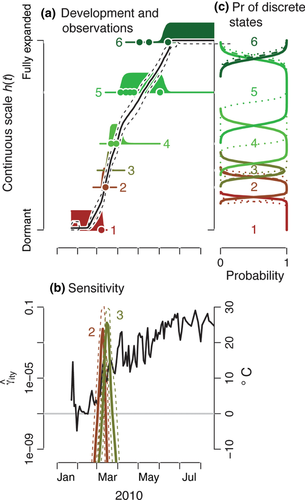
Predictors in the model are daily average temperature, seed source, temperature-seed source interactions, and chilling units. Temperature is an individual/day-scale variable. Seed source is an individual-scale variable, making the temperature-seed source interaction also individual and day. Seed source is a factor for geographic sources north vs. south of the 40°N parallel. Chilling units is an individual and year scale variable, taking to be chilling units accumulated during the preceding winter (Supplement). Soil moisture and vapor pressure deficit were monitored but they do not explain spring phenology in our region, because soil moisture remains near field capacity throughout the time of spring development. Summer droughts do occur, but detectable effects are limited to fall phenology, not spring. This observation is consistent with other studies of spring phenology in moist temperate regions (Cleland et al., 2007). Snow cover was not included because snow was correlated with temperature in this study. Unlike weather station data, which would show large temperature fluctuations throughout winter, our sensors are within the same chambers and at the same heights as plants. Temperatures remain nearly constant during the period of snow cover. Station temperature data would miss this relationship.
Any model can only provide a crude representation of how variation in temperature affects a cumulative process, such as spring phenology. However, the common thermal (degree-day) models and regression models summarize the entire process by one aggregate number for a season or year, the CDM is more sophisticated, but still simple. The ‘memory’ in the model is the changing state of the organism h(t), which responds to all fluctuations in temperature. Development can commence when a threshold is reached, accelerate on warm days, and decline to zero on cold days. Temperate effects can interact with other environmental variables and attributes of the individual. These effects of daily responses culminate in a discrete event (budbreak), but the entire history of fluctuations control the event, rather than a single number.
We evaluate the three ways to quantify effects of warming using experimental data. We describe the experimental methods followed by application of a new (CDM) to identify timing of warming effects and how they vary within and between species.
Experimental methods
Experimental warming was implemented at two sites, one each in the southern and northern ranges of North America's eastern deciduous forest. The southern site, Duke Forest (DF), is near Hillsborough, North Carolina (36.0°N, 79.1°W; elevation 180 m) and has a mean annual temperature of 14.5 °C and annual precipitation of 1208 mm, nearly all of which falls as rain. The northern site, Harvard Forest (HF), is in Petersham, Massachusetts (42.5°N, 72.2°W; elevation 340 m), and has a mean annual temperature of 7.5 °C with 1183 mm of precipitation. At Harvard Forest, snow cover is typical from December to March.
The experiment used a factorial design to provide replication of three chambers each for all combinations of three temperatures (ambient, ambient + 3 °C, and ambient + 5 °C), and two light levels (gap and understory) for a total of 18 chambers per site. Individual responses to warming treatments were tracked by following seeds through germination and growth, with a special focus on phenology. Air and soil were directly and independently heated.
At each site, we created an artificial gap in the summer of 2008 by removing all trees with minimal soil disruption. Within each gap and intact-canopy stand, we constructed nine rectangular open-topped chambers measuring 5.1 m × 3.2 m. Within each chamber, two 4.6 m × 1.05 m areas were designated as ‘experimental strips’ for soil heating and seed establishment. Chamber walls consist of transparent plastic greenhouse sheeting attached to wooden frames, with heights of 2.5 m in the gap and 1.5 m in the understory to accommodate different growth rates in the two locations. Three temperature treatments, designated ambient, +3, and +5 were randomly assigned to the chambers within gap and understory light treatments. Three additional control plots had no chamber but did have coarse mesh fencing to exclude large herbivores.
Soil and air were heated with independent systems to track ambient temperatures with the consistent +3 °C and +5 °C offsets. Soil was heated with electric resistance cable buried 10 cm deep at 20 cm spacing (Melillo et al., 2002). Temperature offsets were maintained by an automated tracking system. Ambient chambers received buried cables as a disturbance control, but they were not heated. Air was heated indirectly with propane. Heated water with nontoxic propylene glycol was pumped to a heat-exchange coil and air-flow system in +3 and +5 chambers. Air circulating through the ambient chambers was not heated. The temperature offset was maintained by a defined heat delivery rate. By tracking ambient temperatures, warming treatments contain the same fluctuations in temperature, but simply translate them to a larger mean.
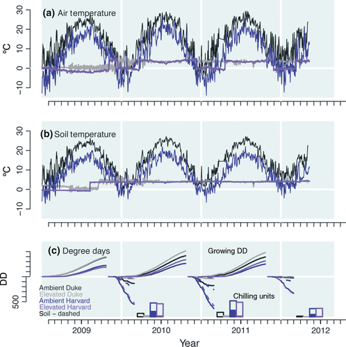
Environmental variables monitored in each chamber included soil and air temperatures. Control of soil temperature in the heated chambers was excellent (±1 °C of target), whereas control of the air temperature was less precise, in part due to air scooping on windy days (Fig. 2).
The 17 m2 rectangular chambers were gridded into 14 columns and 30 rows at 15 cm spacing, resulting in 420 planting locations along an unplanted access. Cohorts were established annually from seed, beginning in 2009, obtained from sites across eastern North America. For purposes of seed provenance analysis, they were classified as northern and southern source, defined by 40°N latitude. A summary of species, numbers of individuals by species and source populations, and numbers of observations per individual are summarized in Table 1. Seeds from each source were planted in equal numbers at each site. Planting occurred at the times of seed dispersal for each species in the mineral soil horizon at grid locations. Each year existing cohorts were amended with new planting, replacing losses due to death and selective harvest for analysis. Naturally recruited seedlings were also marked and monitored at both sites.
| Species | Model | Number of trees | Tree years | Number of populations | |
|---|---|---|---|---|---|
| Southern | Northern | ||||
| List | – | 124 | 383 | 4 | 0 |
| Beal | Chill | 344 | 950 | 0 | 3 |
| Bepa | Chill | 123 | 359 | 0 | 1 |
| Litu | Chill | 311 | 933 | 6 | 1 |
| Magr | Chill | 69 | 153 | 2 | 1 |
| Pipa | Chill | 40 | 105 | 3 | 0 |
| Pire | Chill | 62 | 196 | 0 | 1 |
| Pita | Chill | 283 | 838 | 3 | 0 |
| Acru | Chill seed T X seed | 1649 | 4260 | 4 | 3 |
| Acsa | Chill seed T X seed | 191 | 391 | 5 | 3 |
| Fram | Chill seed T X seed | 161 | 321 | 4 | 3 |
| Nysy | Chill seed T X seed | 148 | 339 | 5 | 3 |
| Pist | Chill seed T X seed | 241 | 685 | 2 | 3 |
| Qual | Chill seed T X seed | 980 | 2659 | 5 | 2 |
| Quru | Chill seed T X seed | 246 | 622 | 4 | 4 |
Weekly censuses enabled us to quantify germination, demographic, and phenological responses to warming in each experimental year (2009–2012). The opening of buds and development of leaves in the spring were scored on a scale of 1 (no bud activity) to 6 (fully hardened and expanded leaves)(Norby et al., 2003). The six discrete stages of phenological development are included in Table 2. These stages were assigned to each individual at each census. Phenology observations included in the analysis omit the germination year, to avoid effects that could be related to the precise timing of planting and germination. Seed source was a predictor only for individuals having at least 10 survivors from three or more populations both north and south. Whether or not seed source was including in the final model was determined by model selection (and whether or not sufficient seedlings survived from enough sources).
| Stage | Hardwoods | Conifers |
|---|---|---|
| 1 | No visible bud swelling | No bud expansion |
| 2 | Bud swelling | Stem elongating |
| 3 | Bud break has occurred | Needles have emerged from sheathes |
| 4 | Leaves unfolding | Needles partly elongated |
| 5 | Leaves open, not fully expanded | Needles mostly elongated but unhardened |
| 6 | Fully expanded | Needles hardened |
Temperatures, growing degree days, and chilling units for the experimental chambers are shown in Figure 2. Growing degree days accumulate over the season. In degree-day models, a degree-day value is used for the date on which an event occurred (e.g., budbreak), representing the sum of daily temperatures above a threshold value.
The chilling requirement was evaluated according to standard practice for degree-day models, as the accumulated temperatures below a threshold temperature of 0 °C (e.g., Linkosalo et al., 2006). The degree-day sums are shown with temperature by site and year in Fig. 2c. Chilling units are defined as the sum of daily temperatures below a threshold taken up to 1 January. Chilling units are large for Harvard Forest, especially in 2011, and small for 2012, exceptionally warm at both sites. The degree days and chilling units in Fig. 2c are examples of aggregate values discussed in the Introduction – they collapse all of the variation in Fig. 2a into a single number for a given year. The CDM uses the full variation provided by all combinations of chambers, sites, treatments, and years. Analytical methods are available in the SI text.
Results
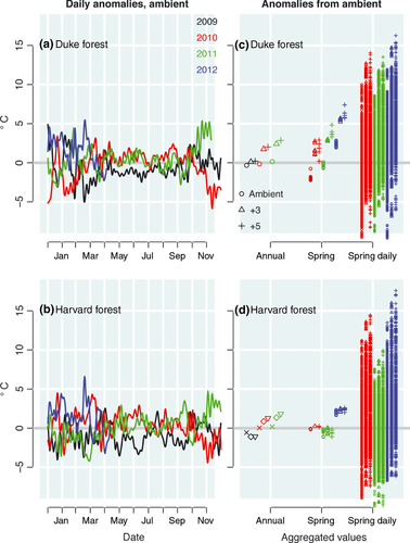
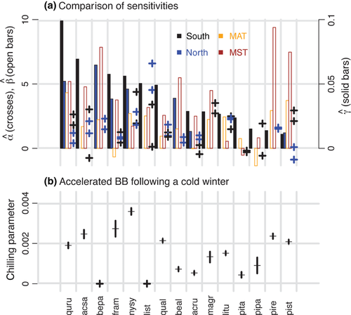
Effects of aggregation on temperature data are dramatic (Fig. 3). To isolate the effect of aggregation, as opposed to the error that comes from using weather data distant from the site, we used temperatures experienced by each plant. Smoothed daily temperatures vary substantially over the 4 years, with the largest anomalies occurring during the critical period of spring development (Fig. 3a, b). This variation does not survive the averaging that results in aggregate values (left side of Fig. 3c, d). The loss of variation through aggregation affects both the mean and variance (eqn S1). By substituting MST for MAT as the predictor, we increase variation (center of Fig. 3c, d), and change estimates (open bars of Fig. 4). Not just the variance but also the mean is changed by the shift from MAT to MST. For example, the year 2010 is warmer than 2011 at Harvard Forest based on MAT, whereas the reverse is true based on MST. Both MAT and MST fail to capture the important variation, clearly evident at the daily scale (right side of Fig. 3c, d). A sense of the effect of these different predictors on slope β is gained from the comparison of regression lines that generate them in Fig. S2. Estimates are summarized in Table S1, based on MAT and MST.
 (3)
(3)The CDM identifies large species differences. The variables contained in the selected model, based on DIC, are shown in Table 1. Estimates of γ-sensitivity aggregated at the species level span an order of magnitude (solid bars in Fig. 4a), and they are confidently estimated (Fig. S3a). Spring warming disproportionately advances the growing season for Acer saccharum, Betula papyrifera, Quercus rubra, and Fraxinus americana. γ-sensitivity depends on temperatures of the preceding winter (Fig. 4b) and on interactions with source population (blue vs. black bars in Fig. 4a). With one exception (Pinus strobus) species having a significant seed source effect show greater sensitivity to warming in southern populations. Chilling responses expected from physiological understanding have been difficult to identify (Hänninen et al., 2007; Hänninen & Tanino, 2011). Their effects on continuous development are confidently estimated using the CDM (Fig. S4b). The largest positive values for Acer saccharum, Nyssa sylvatica, and Fraxinus americana suggests that these species might experience unsatisfied chilling requirements during warm winters.
Because we estimate sensitivity by all methods using the same data we can confirm that methods themselves introduce strong biases. α- and β-sensitivity estimates do not agree with one another or with γ-sensitivity (Fig. 4A). The differences in β estimates that come from using MAT vs. MST exceed the average differences between species. In some cases they differ in sign. The disagreement between them, together with knowledge that they cannot discriminate important temperature variation, makes both α- and β-sensitivity hard to interpret. Neither provides information on the timing of temperature variation that controls budbreak.
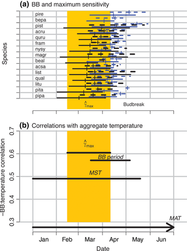
The CDM identifies a critical period in late winter/early spring (Fig. 5a). Each individual follows an arc of temperature response, which increases from low values in autumn through midwinter, and then declines from late winter until the time of BB (Fig. 1b). Maximum values are predicted later at northern sites (blue lines in Fig. 5), and they anticipate the main period of budbreak by several weeks.
Discussion
There are several broad implications for warming climate and phenology that result from a model of continuous responses to temperature coupled with discrete observations. First, the most accurate and rapid prediction tool for future phenology could focus on a specific period in late winter (Fig. 5). The timing will differ regionally, but the generalization holds for our sites in both northern and southern parts of the eastern deciduous forest.
Second, the apparent conflict between experiments and observational studies results from the different ways data are analyzed. Both yield valuable data, but must be modeled appropriately. The changing effect of temperature throughout development is sufficiently diluted and changed by aggregation as to distort relationships. The correlation between MAT and BB is too low to be useful for prediction (Fig. 5b). The upward bias in observational studies relative to experiments is apparent when the different analyses are applied to the same results (β open bars are more often larger than α crosses in Fig. 4a than not), but the loss of information caused by aggregating temperature is not limited to this systematic bias. Our approach can be applied to both; we used experimental data for this application, because it allowed us to compare individuals from the same and different (but known) geographic sources to different combinations of temperature treatment.
Third, clear species differences are resolved (Fig 4 and Fig. S4); in traditional approaches aggregation results in broadly overlapping estimates of response, whereas the CDM finds clear distinction. We have not exhausted all alternative assumptions that could be applied to phenology data. For example, one might test for the correlations between all combinations of vaverage monthly temperatures and budbreak dates. The limitation of such an approach is the fact that it still relies on a highly aggregated predictor for an event that depends on continuous development. We have used several example indices common in the literature (Fig. 3) to make the point that a continuous model avoids the aggregation problem entirely.
Fourth, the CDM captures the effects of variation in a way that can be directly implemented in predictive modeling. Future warming will not occur uniformly throughout the year. For example, the southeastern US, which was been slow to warm on average, has witnessed a large increase in climate variation (Li et al., 2011). The CDM captures this variation and predicts that winter warming can accelerate onset of growth, despite small interannual differences in MAT (Fig. 4B and Supplement). Our approach quantifies these effects under current and experimental conditions and, thus, provides guidance not available from other methods. The CDM approach can be applied as a simple rule-of-thumb predictive interval (Fig. 3) or implemented in models that track daily weather (Fig. 1).
The CDM finding that there is a consistent critical period of temperature variation that differs from currently used indices needs evaluation. If the CDM prediction of critical timing in late winter (Fig. 5a) is correct, then temperatures of this period should be more strongly correlated with BB timing than those based on other intervals. We compared results with temperatures aggregated over the season until the time of BB, as used in degree-day models (Linkosalo et al., 2006; Delpierre et al., 2009; Ibáñez et al., 2010; Morin et al., 2010; Wolkovich et al., 2012) and closely overlapping MST, and with other intervals commonly used in phenology analysis, including MAT and the period when BB is occurring. Although the CDM is calibrated to information throughout the season, and not specifically to BB, we find that it does in fact predict timing better than the traditional indices that are directly calibrated to FO data (Fig. 5B).
Future applications of the model to observational data will extend interpretation to new sites. This first application to experimental data provides opportunity to compare the different methods used to analyze phenology data where both types of analysis can be directly compared.
Acknowledgements
Funding was provided by the US Department of Energy. For comments on the manuscript we thank Anne Stine, Matthew Kwit, Denis Valle, Kai Zhu, and three anonymous reviewers. For field assistance we thank Lindsay Scott, Becky Roper, and Ben Vierra.


