Determination of energy dissipation during cyclic loading and its use to predict fatigue life of metal alloys
Abstract
An approach to determine the specific energy dissipated during cyclic loading of metal alloys with load ratios between 0 and 1 is developed. The dissipated energy per cycle is determined by using a limiting procedure to obtain the area enclosed between successive loading and unloading curves and can be used for low-, medium-, and high-cycle fatigue. Comparisons with published data from two aluminum, one titanium, and one steel alloy show that the predictions capture the test results very well. A universal curve relating cycles to failure to two nondimensional parameters is derived. It is shown, in some limiting cases, that the method leads to power law equations with the parameters in these equations determined directly from the complete stress–strain curve of the material with no need to fit experimental data. Furthermore, if certain conditions are satisfied, the method is consistent with the existence of an endurance limit and Miner's rule.
Highlights
- Model describing the shape of loading and unloading curves during fatigue is developed.
- A closed-form expression for the fatigue cycles to failure initiation is obtained.
- A single master curve for fatigue is created in terms of two variables.
- Comparisons with test results for four alloys show good to excellent agreement.
1 INTRODUCTION
The concept that fatigue failure occurs when the total energy dissipated during cycling equals the available energy per unit volume, that is, the area under the stress–strain curve, has been around for almost 100 years. As early as 1927, Inglis1 was among the first to propose this approach. He was followed by other investigators2, 3 who attempted to develop the concept further. Manson4 and Coffin5 related the cycles to failure to the width of the hysteresis cycle, and Halford and Morrow6 proposed a closed-form expression for the energy dissipated per cycle applicable to low cycle fatigue. Their approach was extended to medium and high cycle fatigue by Chang et al.7
Examining the relationship between hysteresis and the rate at which damage accumulates during cyclic loading, Erber et al.8 established phenomenological relations between energy dissipated during hysteresis and cycles to failure. These were linked to earlier work mentioned above but also established a framework for further experimental and simulation work. Within this framework, Tchankov and Vesselinov9 used an incremental approach to calculate the total hysteresis energy for random applied loading and applied it to predict fatigue failure on a steel alloy.
Constantinescu et al.10 provided an analysis that is equally applicable to low- and high-cycle fatigue by providing an interpretation of elastic shakedown in terms of dissipated energy. Charkaluk et al.11 established a damage indicator based on the energy dissipated per cycle using a viscoplastic stress–strain law and three-dimensional finite element simulations.
An attempt to relate energy dissipated per cycle to the creation and propagation of random microcracks in the material was made by Troshchenko.12 To further understand energy dissipation, Meneghetti13 developed a model to relate the heat loss per cycle per unit volume to cycles to failure and applied it to a steel alloy. Korsunsky et al.14 derived an expression for the dissipated energy per cycle under fully reversed loading for a Ramberg–Osgood-type alloy, which is very similar to the expression derived by Halford.15 They also compared the accuracy of the energy dissipation criterion to two other methods and showed that it is more reliable.
Scott-Emuakpor et al.16 observed that dividing the monotonic strain energy to failure by the average strain energy dissipated per cycle may not be sufficient if it is necessary to account for the experimentally observed increase of the strain energy dissipated per cycle near the end of life. They carried out experiments on an aluminum alloy and showed an exponential increase of the strain energy dissipated per cycle near final failure. Park et al.17 studied the effect of twinning and de-twinning during low cycle fatigue loading of a magnesium alloy and found that the plastic energy dissipated per cycle correlates well with the cycles to failure.
A numerical approach to calculate the instantaneous energy dissipated per cycle under thermomechanical fatigue loading was introduced by Gosar and Nagode.18 One of the advantages of this approach is that it can calculate energy dissipated at any point during a cycle and not after each cycle is completed as most other methods do. Liakat and Khonsari19 used a finite element approach to calculate the entropy generated and plastic energy dissipated during tension–compression fatigue loading and compared to test results. They showed that the energy generated due to heat conduction was negligible compared to the plastic strain energy.
Fan et al.20 examined the effects of creep and stress relaxation on fatigue life. They found a power law relation between generalized hysteresis energy and fatigue life of a 316L(N) alloy. Within the same context of fatigue creep interaction, Wang et al.21 proposed a creep-fatigue model using a modified model based on the dissipated strain energy per unit volume and applied it to a number of steel alloys with satisfactory results. An evaluation of the dissipated energy approach for AISI 316L alloy under multiaxial fatigue was carried out by Feng et al.22 and showed that, overall, it was superior to models based on the critical plane approach.
All previous works have demonstrated that the dissipated strain energy per unit volume, or energy density, accumulates during cycling as long as there are plastic strains present. And when the total energy accumulated equals the static total energy, the area under the stress–strain curve, fatigue failure occurs. Several issues remain such as the fact that the total plastic energy may change over time and with loading type. In general, most methods rely on a combination of experimental results and simulation to determine the energy dissipated during each cycle and are mostly applicable to low cycle fatigue where the plastic strains are most pronounced. The fact that the dissipated energy changes as a function of cycles and the difficulty to determine its stabilized or limiting value adds to the difficulty of correlating the dissipated energy density with fatigue life.
In this work, an approach to estimate the energy dissipated per cycle is proposed using some basic phenomenological properties of the loading and unloading cycles. The resulting closed-form expression for the dissipated energy is shown to have a finite limit as the number of cycles increase. This limit is divided into the total static strain energy density to obtain accurate fatigue life predictions for low, medium and high cycle fatigue.
2 APPROACH
2.1 Tension–tension fatigue with 0 ≤ R < 1
We start with the case σmin/σmax = R = 0 because it is easier to introduce the assumptions and the basic equations. After that introduction, we will generalize to any positive R value. The case of R = 0 will then follow from the derivation as a special case.
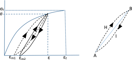
In addition to the static stress–strain curve to failure, the first two unloading–reloading cycles for R = σmin/σmax = 0 are also shown in Figure 1 with residual plastic strains εm1 and εm2, respectively. The area enclosed in each unloading–reloading cycle is the specific energy dissipated in that cycle and will be determined first. To proceed, the following assumptions are made (see right portion of Figure 1):
- Each loading cycle is described by a corresponding Ramberg–Osgood stress–strain law as in Equation (1) with, in general, different values for the starting slope Ei, coefficient Ki and exponent ni. In what follows, it will be assumed that the starting slope of the loading cycle Ei is the same as Eo.
- The loading curve AHB has the same slope as the original stress–strain curve at point B with coordinates (ε, σ).
- The area between the straight line AB connecting (εmi, 0) with (ε, σ) and the unloading curve BIA is the same as the area between line AB and the loading curve AHB. That is, the straight line AB divides the unloading–reloading cycle in two approximately equal regions.
- It is assumed that the areas of the delineated regions obey the relation:
We now generalize to any positive R value less than 1. This is shown in Figure 3.
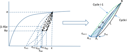
- The shape of the unloading curve for R = 0 is the antisymmetric of the shape of the loading curve for the same cycle with center of (anti-)symmetry the mid-point of AiB.
Since σ/Eoε can only vary between 0 (no applied load) to 1 (material response is perfectly elastic), Equation (40) can be plotted in Figure 4. It can be seen from Equation (40) and Figure 4 that if there is a portion of the stress–strain curve, which is perfectly linear, then, for that portion, σ = Eoε, and the fatigue life is infinite. The highest value of σ for which σ = Eoε would then be the endurance limit for this material. This transition from perfectly linear to nonlinear behavior emphasizes the importance of very accurate strain measurements during a stress–strain test as deviations from linearity that are a small fraction of a percentage point could make the difference between infinite and finite fatigue lives. This will be addressed below when physical interpretations of σ/(Eoε) are discussed.
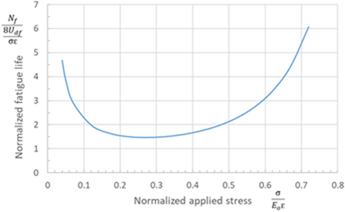
Another interesting implication of Equation (40) is the existence of a minimum of the right hand side. It occurs when σ/(Eoε) = 0.2711 and leads to a minimum value of the normalized cycles to failure (left hand side of Equation (30)), which is 1.4716. Such values of σ/(Eoε) are, typically, deep into the plastic range and result in low cycle fatigue.
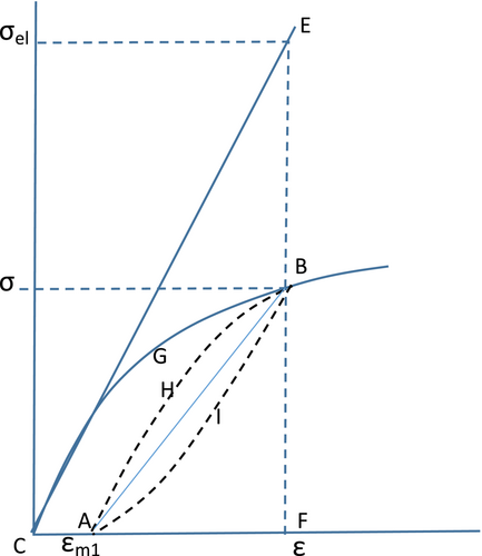
This is the ratio of the energy density of a linear material loaded to (ε, σ) to the energy density (area of triangle CEF in Figure 2) that would be stored in the actual material if it behaved linearly with Young's modulus Eo when strain ε were applied. This is related to Assumption 4 made earlier and emphasizes that the dissipated energy and, through it, fatigue life depend on ratios of available and “unavailable” energies with the word “unavailable” referring to fictitious behavior that the material might exhibit if it were linear or had no plastic residual strains. It also shows that, according to Equation (40), the life would be infinite if there were no plastic strains, that is, if σ = Eoε. This has been postulated and observed in the past with Coffin,5 among the first to suggest that plastic strains are necessary for finite fatigue lives and that such plastic strains imply that an endurance limit does not exist.
Another way to view this quantity, σ/(Eoε), is as the ratio of elastic strain σ/Eo to the total strain ε. This becomes particularly interesting when the term (1 − σ/(Eoε))2 at the denominator of Equation (40) is considered. If the elastic strain σ/Eo is close to the total strain ε, the quantity 1 − σ/(Eoε) is close to zero, and its square becomes very small. In such situations, this term in the denominator of Equation (40) dominates, and very long lives are predicted. Because of this strong nonlinearity of the cycles to failure, very small changes in the value of ε lead to very large changes in the fatigue life. For example, if σ/(Eoε) equals 0.95, and the value of ε changes by about 4% to 0.99, the resulting fatigue life increases by a factor of 25. This makes very accurate knowledge of the applied total strain ε extremely important as, for high cycle fatigue, especially close to the endurance limit, differences in that value of even 1%, when σ/(Eoε) is close to 1, have a large effect on the fatigue life. This sensitivity is also responsible for the large fatigue scatter. On the one hand, nominally identical specimens will easily have variations in the stress–strain curve, which, near the linear region, will easily exceed 1% since the coefficient of variation for Young's modulus of most alloys is in the range 4%–6%. On the other, applying the exact strain (or stress) in an experiment can be a challenge if this kind of accuracy is to be maintained. Small variations will lead to large changes in fatigue life. Based on this discussion, one would expect the fatigue scatter to be higher at lower applied loads and this is borne out by test results.
This sensitivity to the term (1 − σ/(Eoε))2 brings up an interesting trade-off. For materials with high plastic strain capabilities loaded with high plastic strain, this term is close to 1, but the area under the stress–strain curve Udf can be quite high. On the other hand, for materials which are nearly linear, this term is very close to 0, which would increase the cycles to failure, but Udf is very low. It is the “right” combination of area under the curve Udf and material nonlinearity, which will lead to the longest lives.
Finally, it is easy to show that Miner's rule follows naturally from the formulation. If different stress levels are applied for different numbers of cycles, each would dissipate a certain amount of energy miUdf/(TΔA)i, following Equation (38), with mi the number of cycles with per cycle dissipated energy (TΔA)i. If these amounts add up to Udf, there is failure. Implicit in this is that the stress–strain curve and, more importantly, the amount of energy dissipated per cycle do not change or any changes have negligible effect on the dissipated energy in the stabilized cycle given by Equation (37). It is recognized here that the equations derived so far, are for stabilized fatigue cycles and neglect the cycles and energy dissipated up to stabilization. Tests have shown that Miner's rule does not always hold and improving the energy dissipation calculation to account for changes during fatigue loading would be a needed refinement.
It should also be noted that the approach can be extended relatively easily to apply to cases with R < 0 provided compressive stress–strain curves of sufficient accuracy are available.
3 COMPARISON WITH TEST RESULTS
As was already discussed, the proposed method requires non-zero plastic strains. As such, it would not work in the linear elastic region of a material unless it is assumed that no material has a perfectly elastic region and there are tiny deviations from the linear behavior, which may not be easily measurable but may be sufficient to create plastic strains. This means that very accurate measurements of the complete stress–strain curves of a given material would be needed. It was already mentioned that small errors in strain measurements lead to large changes in predicted fatigue lives. Thus, the accuracy of extensometers and strain gages, even the thickness of lines used to plot stress–strain curves will have a significant effect on the predictions. As a result, an attempt was made to create a consistent approach to translate published stress–strain curves to data usable in the present approach.
The advantage of this equation is that it acts as complementary to the Ramberg–Osgood relation, which has the strain on the left hand side. It is recognized here that there are published values for the Ramberg–Osgood constants K and n; however, these are meant to go deep into the plastic regime and may not be as accurate in the nearly linear region where the present method is most sensitive.
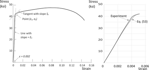
It should be noted that A from Equation (55) is always negative. Then, for a number of strain values εi (at least four) between 0 and εy, the corresponding stress values, σi, can be obtained from Equation (53), and Equation (1) is best fitted through the pairs (εi, σi) to obtain K and n for strains in this range. An example of this is shown in Figure 5 for 6061-T6 aluminum with the stress–strain curve taken from fig. 3.6.2.2.6(m) in literature.25 The portion with low applied strains up to εy is also shown (zoomed in) on the right of Figure 5 showing that the difference between Equation (53) and experiment is very small and only in the vicinity of εy. If the applied strain is greater than εy, it can be read directly off the stress–strain plot for the material and used in Equations (38) and (39) to predict fatigue life. As this strain is significantly greater than the elastic strain, any errors in its exact value, which would be an issue for lower applied strains, lead to small changes in the predicted fatigue lives.
Predictions of Equations (38) and (39) were generated for four alloys, 7075-T6 aluminum, 6061-T6 aluminum, Ti 6-4 titanium, and 4340 steel, and were compared to test results from literature.25 Stress–strain curves given in literature25 were used to obtain Eo, σy, and εy. Udf was obtained by numerical integration of these stress–strain curves. K and n were obtained using the procedure described above via Equations (53) to (55). The values of these variables are summarized in Table 1. Note that, for R ≠ 0, n1 in Equation (38) was obtained from Equation (32) using n from Table 1.
| Property/material | 7075-T6 Al | 6061-T6 Al | Ti 6-4 | 4340 steel |
|---|---|---|---|---|
| Eo (GPa) | 71.60 | 67.80 | 116.5 | 201.1 |
| Udf (MPa) | 65.01 | 45.48 | 100.05 | 193.7 |
| εy | 0.0097 | 0.0052 | 0.01025 | 0.0065 |
| σy (MPa) | 579.1 | 294.4 | 947.9 | 1206 |
| Sy (GPa) | 4.387 | 4.136 | 6.204 | 147.7 |
| A (Pa) | −2.716 × 10¹⁹ | −5.719 × 10²⁰ | −3.338 × 10¹⁷ | −3.512 × 10¹⁵ |
| α | 5.648 | 5.688 | 4.59 | 3.449 |
| K | 1.564 × 10⁹ | 5.470 × 10¹² | 3.414 × 10⁷ | 9.705 × 10⁴ |
| n | 5.90 | 5.76 | 5.03 | 3.74 |
The predictions by Equations (38) and (39) are compared to test results from literature25 for 7075-T6 aluminum for R = 0 and R = 0.5 in Figure 6. For the R = 0 case, the test data include enough points to give an indication of the scatter. For this case, the predictions of the present method for the 1 and 99 percentile curves are also shown. These are obtained by treating εy as a normally distributed variable and using statistical data from literature,25 namely, the A-Basis and B-Basis values, to backcalculate a coefficient of variation. The mean curve slightly overpredicts and the predicted scatter band contains most of the data. For R = 0.5, the predictions are higher than test results by at most a decade on the cycles axis. The predictions for 6061-T6 aluminum for R = 0 and R = 0.5 are shown in Figure 7. Very good agreement with test results is observed for R = 0. For R = 0.5, the trend is captured very well but the predictions are higher than the tests again by at most a decade on the cycles axis. The predictions for titanium 6-4 for R = 0.01 are shown in Figure 8. There is very good agreement with the test results. Finally, The predictions for 4340 steel for R = 0.2 and R = 0.54 are shown in Figure 9. In both cases, the predictions are in good agreement with test results.


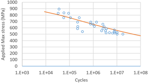

Overall, the predictions follow the trends from the experiments very well for all four alloys and for R = 0 are in very good agreement with test results. For the case where there were sufficient test data, the scatter band predicted by the present method also is in reasonable agreement with the scatter observed in the test results.
4 SUMMARY AND CONCLUSIONS
A method was developed to determine the energy density dissipated during each fatigue cycle in a metal alloy and was used to predict fatigue life up to damage initiation for cases with 0 ≤ R ≤ 1. The resulting expressions for cycles to failure are in closed form and make no use of parameters fitted to experimental results. Only accurate static stress–strain data are needed. The method was shown to degenerate to standard power law equations with the coefficient and exponents in those equations determined directly from the complete static stress–strain curve. It was shown that nonlinear strains must be present for finite fatigue lives, and if a portion of the stress–strain curve is perfectly linear, the fatigue life is infinite for that portion suggesting ways to determine an endurance limit (if the material has one). Comparison of predicted fatigue lives with test results for two aluminum, one titanium, and one steel alloy showed good to very good agreement with tests.
The proposed method is very promising, but it relies on a number of assumptions the validity of which needs to be further examined. (1) Almost the entire stress–strain curve must be nonlinear. For low applied strains, there is great sensitivity to the value of the quantity σ/(Eoε) and very small errors in that value lead to great changes in the predictions. This on the one hand emphasizes the need to measuring strains to an accuracy better than ±50 μs and on the other points to an inherent source of fatigue scatter: Nominally identical specimens will have very different fatigue lives if they have small differences in this value. (2) The formulation is based on a Ramberg–Osgood-type material. As such, the stress–strain curve must be monotonically increasing. This means that materials with significant necking would not be captured by the model if fatigue lives for applied strains past the maximum of the stress–strain curve are needed. All four alloys examined here exhibit some amount of necking. For this reason, the predictions were kept to strains below the point where necking starts and the results are still accurate. (3) It is assumed that the static stress–strain curve does not change with fatigue cycling. This is an approximation as localized extended plasticity may cause load redistribution not captured by a single stress–strain curve meant to represent an entire specimen throughout its fatigue life.
When applied to load ratios R ≠ 0, the method has the tendency to overpredict test results. This requires further investigation. A single “master” curve for predicting cycles to failure can be constructed and shows that, within the framework of the assumption made, two parameters, σ/(Eoε) and Udf/(σε), are sufficient to describe the behavior.
Open Research
DATA AVAILABILITY STATEMENT
The data that support the findings of this study are available in Department of Defense Handbook, Metallic Materials and Elem at https://automaterials.files.wordpress.com/2018/09/military-handbooks-a-collection.pdf. These data were derived from the following resources available in the public domain: Department of Defense Handbook, Metallic Materials and Elem, https://automaterials.files.wordpress.com/2018/09/military-handbooks-a-collection.pdf.


