Effects of non-proportionality and tension–compression asymmetry on the fatigue life prediction of equivalent stress criteria
Abstract
Biaxial tension/compression–torsion fatigue tests with varying levels of non-proportionality were performed employing a structural adhesive designed for wind turbine rotor blades. The cycles to failure were found to be independent of the level of non-proportionality. It is demonstrated that numerical fatigue life predictions via rainflow-counted equivalent stress histories are not able to replicate these experimental observations and overestimate the fatigue life up to a hundredfold. The tension–compression asymmetry of the adhesive resulted in significant damage prediction differences depending on the stress space representation of the Haigh diagram. If not properly taken care of, the asymmetry will also lead to non-conservative results. While demonstrated with a short fiber-reinforced adhesive, the results can be transferred to other materials.
Highlights
- Non-proportional fatigue tests employing a structural adhesive.
- The cycles to failure were found to be independent of the level of non-proportionality.
- A tension–compression asymmetry significantly influences the fatigue life prediction.
- Rainflow-counted equivalent stresses overestimate the non-proportional fatigue life.
1 INTRODUCTION
Fatigue damage modeling is usually based on uniaxial experimental data. However, multiaxial fatigue loads are very common in engineering applications. To allow for a broader understanding of multiaxial fatigue phenomena, these also have to be replicated in experiments. This way, the reliability of (multiaxial) fatigue damage models can be validated.
Among multiaxially loaded components, different loads can be independent of each other, which can lead to varying principal stress–strain directions. This load state is classified as non-proportional and can cause additional uncertainties with fatigue life predictions.1, 2
Depending on the material, the same load amplitude can lead to different cycles to failure in a non-proportional load state compared to a proportional one. Sonsino3 showed that ductile materials tend to exhibit a decreased fatigue life in non-proportional loads, while brittle materials can show increased fatigue life.
Independent of the altered cycles to failure, fatigue analyses for non-proportional loads require additional care, because of the potentially lower damage prediction quality of standard methods, such as the evaluation of rainflow-counted equivalent stress histories.1, 2
One way to recreate non-proportional loads in experiments is to use tension/compression–torsion testing machines with a phase shift in between the sinusoidal normal load and the sinusoidal torsional load. Due to the complexity of the test setup and challenging tubular specimen manufacture,4 non-proportional experiments on polymers5, 6 and other materials7-10 are rather scarce in literature and non-existent in terms of structural adhesives for wind turbine rotor blades, yet.
Rotor blades of wind turbines are among the largest and most heavily loaded components of any kind. Due to their vast size and the stochastic nature of the wind, each blade experiences a 3D wind field and thus a stochastically varying wind load with each rotation. This wind load is superimposed with a gravitational load based on the rotation of the rotor, which is approximately sinusoidal and smoothed by the large inertia of the complete rotor.
The combination of the stochastic wind load and approximately deterministic gravitational load leads to complex multiaxial fatigue stresses, which can exhibit significant levels of non-proportionality depending on the blade design and average wind speed.11, 12 While these stress states are dominated by normal stresses due to bending in case of a high blade stiffness, modern rotor blades tend to be more flexible to limit bending stresses. Passive load control features such as bend–twist coupling13, 14 also introduce higher torsional loads in order to limit bending loads. These developments contribute to a more significant influence of multiaxial and non-proportional load states.
In order to simplify the manufacturing, rotor blades of wind turbines are typically made using two aerodynamic half shells and shear webs, which are joined employing structural adhesives. As pointed out in Eder et al,15, 16 the complex multiaxial fatigue loads in the adhesive joints proved to be a design driver for rotor blades.
Therefore, enhanced understanding of the influence of multiaxial and non-proportional loads on the fatigue life of rotor blade adhesives can help to optimize rotor blades. This applies to the experimentally observed fatigue life and equivalent stress-based predictions thereof, since this methodology is frequently used in wind energy contexts.16-21
In this work, the influences of multiaxial non-proportional loads and tension–compression asymmetry on the fatigue life (prediction) are demonstrated by combined tension/compression–torsion experiments. The material under investigation is a structural adhesive commonly used in wind turbine rotor blades. However, general findings and discussions on the fatigue life prediction are not limited to this particular material. Virtually defect-free specimens and a large number of tests maximize the reliability of the results.
Section 2 specifies the material system, specimen manufacturing and test setup. The influence of non-proportional loads on the experimental fatigue life is shown in Section 3 followed by a discussion on the implications of a tension–compression asymmetry on the fatigue life prediction in Section 4. A Haigh diagram is constructed in Section 5, which is subsequently used in the multiaxial and equivalent stress-based fatigue life prediction in Section 6.
2 EXPERIMENTAL SETUP
The manufacturing of the utilized specimens and fatigue testing conditions are briefly explained in the following.
2.1 Material system
In this work, an epoxy-based and short glass fiber-reinforced adhesive is analyzed. As in previous studies4, 22, 23 of the authors, EPIKOTE™ Resin MGS™ BPR 135G3 and EPIKURE™ Curing Agent MGS™ BPH 137G are used. The two-component structural adhesive is commonly used in the wind energy industry. Detailed material properties can be found in the data sheet24 and the aforementioned studies by the authors.
2.2 Specimen design and manufacturing
The specimen design and manufacturing process were optimized in a previous study.4 The specimen geometry is a tapered tube, which was optimized in a finite element-based parametric study in such a way that stress concentrations were minimized. Vacuum speed mixing was combined with 3D-printed mold inserts in an injection molding process to assure a high mixing homogeneity and low porosity level.
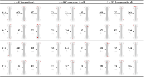
Subsequent to the manufacturing, the specimen quality was analyzed employing high-resolution X-ray microscopy ( CT scanning) using a Zeiss Xradia 410 Versa.25 Qualitative porosity scans are shown in Figure 1 for all specimens in this work. Similar to previous studies,4, 22, 23 the porosity level is negligible in the test section. Only a small amount of pores was found at the end and outer perimeter of the tapered section. These pores are a result of race tracking effects, that is, slight differences of the cross-sectional flow speed distribution during the injection process. However, these pores do not influence the load distribution in the test section on account of their small size and distance to the test section.
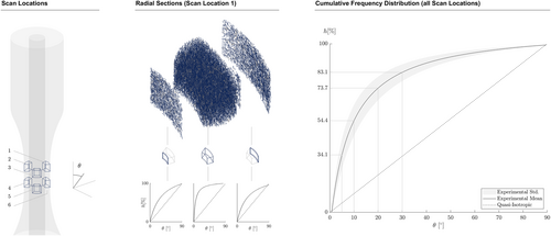
Based on the anisotropic stiffness properties derived in a previous publication4 and additional (very) high-resolution CT scans, the specimens can be classified as transversely isotropic with a large majority of fibers aligned in axial direction. Cumulative frequency distributions of the fiber orientation are shown in Figure 2. Therein, is the angle between the longitudinal axis of the specimen and the axial orientation of the individual fibers. On average 73.7% of all fibers within the scanned areas exhibit an axial orientation with less than 20° deviation to the longitudinal axis of the specimen. Within a distance of 0.25 mm from the inner and outer perimeter, the fiber orientation is closer to a quasi-isotropic distribution (linear dashed lines in Figure 2). Therefore, the fiber orientation is linked to the injection speed, which is lower in close proximity to the mold due to friction. Due to the excellent manufacturing quality of the specimens and the low standard deviation of the results observed in previous studies,4, 22, 23 it is expected that the fiber orientation is approximately the same in all specimens.
2.3 Biaxial fatigue testing campaign
The biaxial (tension/compression–torsion) fatigue tests were performed with a servohydraulic Walter + Bai LFV 100-T200026 equipped with a class 0.5 calibrated load cell. In situ surface temperature measurements were conducted using Pt100 sensors. In addition, the test frequency was adjusted at each load level to limit internal heating of the specimens and strain rate effects on the different load levels.
Two load levels were chosen in such a way that the specimens fail in between 104 and 105 cycles. This way, the specimens fail close to the yield point of the material23 in terms of an equivalent stress amplitude. The level of non-proportionality was adjusted using a phase shift in between the axial and torsional load. A phase shift of ° represents a completely proportional load state and ° approximates a completely non-proportional load state in this work. Based on the results in Noever-Castelos et al,12 it was decided to test intermediate states of ° and ° as these are very common in rotor blade bond lines in contrast to completely non-proportional states. Note that the level of non-proportionality is also related to the blade design, since the design decisions affect the multiaxial stress distribution.
To assure a reliable statistical evaluation of the results, each phase shift (0°, 30°, 60°) on each load level was tested with six specimens leading to 36 specimens in total.
The tests were intended to be load controlled. However, this was not possible in torsion on account of an issue with the inertia compensation of the torsional load cell, which was also apparent in the uniaxial tests of a previous study.22 Therefore, only the axial component was load controlled, and the torsional component was displacement controlled. Both the axial and torsional components were applied as fully reversed loads. On account of the displacement control in torsion, the applied shear stress is not constant, but a collective with roughly 5% degradation. However, this did not significantly change the level of non-proportionality as the phase shift was still constant throughout the tests. The maximum change in non-proportionality was estimated at 2.96% (at Load Level 1 and °) according to the non-proportionality factor proposed by Meggiolaro and de Castro.27
3 INFLUENCE OF NON-PROPORTIONAL LOADS
In this section, the experimental results and a classification of these with respect to literature are described.
3.1 Experimental results
The cycles to failure were found to be independent of the level of non-proportionality. This is true for the mean and the standard deviation as shown in Figure 3. This neutral behavior must, however, not be mistaken as a reason to neglect non-proportional effects, because these still have a significant effect on the numerical fatigue life prediction quality, which will be shown in Section 6.

The results are summarized in Table 1. On account of the low temperature increase during the experiments and the low overall standard deviation of the cycles to failure, it is expected that temperature-dependent effects can be neglected. The shear stress amplitudes given in Table 1 have to be understood as damage equivalent amplitudes of the shear stress collectives, which resulted from the displacement-controlled torsional load; compare Section 2.3.
| Load Level 1 (L1) | Load Level 2 (L2) | |||||||
|---|---|---|---|---|---|---|---|---|
| N/mm2, N/mm2, Hz | N/mm2, N/mm2, Hz | |||||||
| Specimen No. | [°] | [-] | [K] | Specimen No. | [°] | [-] | [K] | |
| 028 | 0 | 15,238 | 2.12 | 190 | 0 | 46,790 | 4.22 | |
| 200 | 0 | 16,905 | 2.57 | 102 | 0 | 63,182 | 4.15 | |
| 152 | 0 | 16,941 | 2.88 | 016 | 0 | 66,571 | 6.95 | |
| 047 | 0 | 20,467 | 2.88 | 127 | 0 | 80,437 | 4.01 | |
| 074 | 0 | 21,154 | 2.37 | 013 | 0 | 91,302 | 3.20 | |
| 175 | 0 | 28,378 | 3.37 | 032 | 0 | 102,700 | 4.52 | |
| 195 | 30 | 11,665 | 1.63 | 137 | 30 | 48,134 | 5.04 | |
| 156 | 30 | 15,550 | 1.99 | 181 | 30 | 52,560 | 4.46 | |
| 088 | 30 | 16,053 | − | 168 | 30 | 64,048 | 4.54 | |
| 038 | 30 | 17,529 | 1.81 | 044 | 30 | 81,620 | 2.68 | |
| 131 | 30 | 21,312 | 2.56 | 031 | 30 | 92,000 | 2.84 | |
| 157 | 30 | 22,927 | 1.92 | 023 | 30 | 100,900 | 3.35 | |
| 109 | 60 | 15,425 | 2.28 | 185 | 60 | 48,795 | 2.54 | |
| 008 | 60 | 18,134 | 2.34 | 143 | 60 | 65,153 | 2.98 | |
| 095 | 60 | 18,820 | 2.15 | 082 | 60 | 67,440 | 0.90 | |
| 196 | 60 | 19,437 | 2.87 | 049 | 60 | 91,699 | 3.25 | |
| 163 | 60 | 22,943 | 3.70 | 004 | 60 | 98,402 | 3.75 | |
| 079 | 60 | 22,996 | 2.15 | 027 | 60 | 208,500 | 2.18 | |
- Note: Therein, is the test frequency, is the maximum temperature difference to the ambient temperature. A Pt100 sensor failed during the test of Specimen 088 and loosened in case of Specimen 016, increasing on account of friction.
Note that Specimen 027 was treated as an outlier due to a fatigue life of more than double the average. However, this represents a conservative decision regarding the classification of a neutral material behavior in terms of cycles to failure.
3.2 Influence of material ductility
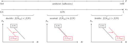
The adoption of the yield strength ratio as a metric for ductility is supported by a discussion on the yield locus of the adhesive presented in a previous publication.23 Therein, the Drucker–Prager32 criterion was identified as a significantly better fit for rather ductile (machine-mixed) specimens in comparison to the von Mises–Schleicher33 criterion, which was proposed for rather brittle (hand-mixed) specimens by other authors.34, 35 Since the Drucker–Prager criterion is more conservative in shear, its yield strength ratio ( ) is lower than that of the von Mises–Schleicher criterion ( ). The applicability of the yield strength ratio as a measure of ductility for the adhesive was thus validated by experiments. Figure 4 visually summarizes the influence of non-proportional loads in combination with the ductility definition explained above. Due to the multiaxiality of the respective – curves, an equivalent amplitude is required. The yield strength ratio of the adhesive ( ) puts it in a neutral category. Given the fatigue results of this study, the observations by Sonsino3 can be confirmed. Since material properties of polymers, for example, the ductility, typically exhibit a strong temperature dependence,36 the influence of non-proportional loads will also be temperature dependent. High temperatures will increase ductility and therefore lead to a reduction of the non-proportional fatigue life observed at room temperature. This effect was also shown by Sonsino.3 Therefore, a temperature related safety factor regarding the permissible cycles to failure seems appropriate to account for different operational temperatures in the field. The magnitude of this safety factor is still to be determined by experiments.
Concerning two-component, fiber-reinforced (rotor blade) adhesives or polymers, the non-proportional effects on the fatigue life will generally be coupled to the fiber distribution and orientation that is achieved in the manufacturing process; compare Section 2.2, because these parameters affect the ductility of the material. This also holds for the curing cycle.
3.3 Fracture surface analysis
The ratio of normal and shear stresses in the experiments was estimated in such a way that their damage contribution is approximately equal in the proportional load case. This is reflected by the main crack orientation of the biaxial tests shown in Figure 5, which was found to be the approximate mean of uniaxial fatigue tests22 in fully reversed axial and torsional loading, respectively.

The main crack orientation was also independent of the level of non-proportionality, that is, the phase shift. This supports the findings regarding the neutral behavior of the adhesive with respect to the cycles to failure, because an altered main crack orientation could indicate a change in the damage mechanism. Simultaneously this highlights the reliability of the manufacturing process,4 as different fiber orientations can introduce different micro- and meso-scale crack orientations.37
4 TENSION–COMPRESSION ASYMMETRY
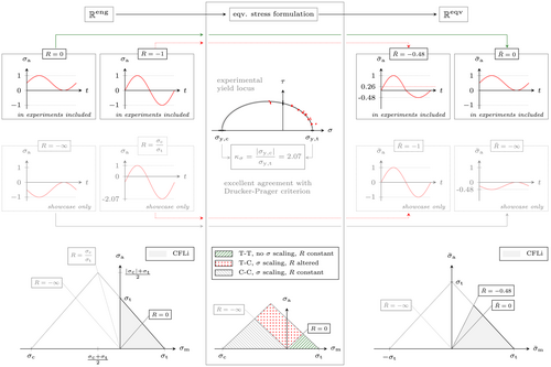
Applying the strength asymmetry of the adhesive to a fully reversed, sinusoidal unit load in results in a 0.26 N/mm2 mean load (peak to peak mean) and a reduction of the stress ratio to in . A fully reversed stress ratio in can be achieved if the stress ratio in resembles the tension–compression asymmetry, that is, . Less complicated conversions are found for pulsating stress ratios. In case of a pulsating load in compression (C-C, e.g., ), the entire load history is compressed leading to smaller amplitudes and mean values in . However, in this case the stress ratio remains constant. A pulsating load in tension (T-T, e.g., ) is not altered at all after the conversion to , since tension stresses already resemble equivalent stresses.
The scaling rules explained above were also transferred to a Haigh diagram at the bottom of Figure 6. Pulsating loads in tension are not scaled, leaving the positions of the respective – lines in the Haigh diagram unchanged. In case of alternating loads, the stress ratio is changed and hence also the position of the respective – lines. For pulsating compressive loads, the stress ratio remains constant. However, as the stress values get scaled, the position in the Haigh diagram also changes, transforming a shifted Haigh diagram in into a symmetric one in .
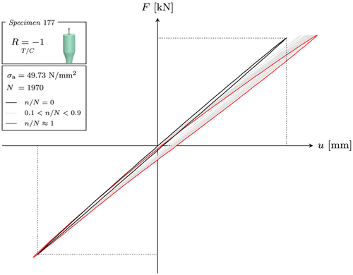
An experimental verification of the tension–compression asymmetry in fatigue is also shown in Figure 7. Therein, the force displacement hysteresis of a uniaxial tension–compression test22 is shown for different ratios between the actual cycles and the cycles to failure . A stiffness degradation is found in the tension quadrant, while virtually no change is observed in the compression quadrant. Thus, a tension stress is proven to exhibit more damage, that is, material degradation, than a compression stress of the same magnitude.
Given that the biaxial (tension/compression–torsion) experiments in this work were done at in , the aforementioned scaling problem in affects the re-calculation of the tests. Hence, a Haigh diagram is required and will be derived in the following.
It should be noted that a tension–compression asymmetry is found for a large variety of polymers38-42 and other materials.43, 44 Therefore, this effect is not unique to the adhesive investigated in this work. In literature, however, implications of the asymmetry on the (equivalent) stress-based fatigue life prediction are hardly considered. This might lead to non-conservative fatigue life predictions, because stresses in are compared to – lines, which are represented in the wrong stress space ( ).
5 HAIGH DIAGRAM
Based on the uniaxial fatigue results recorded in a previous study,22 a Haigh diagram is constructed in the following including a recently proposed – formulation.
5.1 Stüssi–Haibach – approach
The Stüssi–Haibach – approach is a combination of the sigmoidal-shaped Stüssi45 – curve and the Haibach extension line46, 47 in the very high cycle fatigue (VHCF) regime and was proposed in a previous publication.22 Regarding the adhesive, this approach represents an excellent fit of the – data with an engineering approximation for VHCF, as there is not enough data to verify a fatigue limit. Since the Haibach extension line is modeled as a tangent of the Stüssi – curve, a smooth transition between the models is established avoiding the necessity of an arbitrary transition point to be specified by the user. The model is thus easy to use and leads to consistent results. In case VHCF data are available, the slope of the extension line can also be adapted to provide the best overall fit. The approach is visualized in Figure 8.

Afterwards, the extension line is modeled as a tangent to the Stüssi – curve, which was previously fitted to all available data up to the VHCF regime. This way, the remaining variables and can be found. However, if VHCF data is available, the extension line should be fitted to these data instead of using Equation (4) to allow for a better overall fit of the data; compare Figure 8 (Stüssi–Haibach derivates).
In case the – curve has a distinct plateau in the VHCF regime and a drop in fatigue strength beyond that, a combination of the Stüssi – curve with the Sendeckyj49 – curve might also provide a good approximation of the overall fatigue behavior. Shiozawa et al50 among others51, 52 found evidence of such behavior, highlighting the importance of gigacycle fatigue tests.
5.2 Constant fatigue life (CFL) model
Mean stress effects on the fatigue life of a material can be visualized in a Haigh diagram by connecting the available – curves with respect to points of CFL. Depending on the material or the quantity of – curves, different connection line models were proposed.
Therein, and represent an arbitrary stress amplitude and mean stress, while is the stress amplitude of a fully reversed load with zero mean and is the ultimate tensile strength. In case – data for a stress ratio is available, the Goodman approach can be adapted to a piecewise linear interpolation. For simplicity, the piecewise linear approach is chosen for all comparisons and analyses in this work. In addition, the measured – curves are used without any statistical modification. The Haigh diagrams are therefore based on Stüssi–Haibach – curves.
5.3 Model generation and discussion
In Kuhn et al,22 two axial – curves were recorded at and . Wentingmann et al23 determined the tensile strength , which corresponds to .
The resulting Haigh diagram in is shown at the top of Figure 9. It was assumed that maximum amplitudes are found at and that the yield strength ratio is still valid for the ultimate strength ratio. By converting the diagram to , the tension-based results remain unchanged, whereas the – curve at is transformed according to the tension–compression asymmetry; compare Section 4. Therefore, the experimental range in is limited to . As a result, a gap in between and in exists, since experimental data for are not available. Two possibilities were considered to circumvent the -gap, which are shown at the bottom of Figure 9.
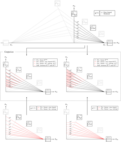
In the first approach, the connection lines in between and are linearly extrapolated. This assumption is based on the overall linearization of the CFL lines in in between the measured (and transformed) – curves. On account of that, the difference of the piecewise linear connection lines to global linear connection lines (traditional Goodman approach) is small for the recorded data in . Therefore, a piecewise linear extrapolation seems to be a reasonable engineering approximation. The linearization effect is also visualized in the mid of Figure 9, where the Haigh diagrams in and are compared. In , the connection lines in between and (in red) are almost a perfect linear continuation of the connection lines between and .
The second approach is based on a conversion of a shear – curve, which was also recorded at in Kuhn et al,22 to using the Drucker–Prager criterion. By employing Drucker–Prager, shear stresses are transformed to equivalent tension values. This conversion is independent of the sign of the respective shear stress, because there is no strength asymmetry in shear. Assuming that the Drucker–Prager criterion can be used in fatigue, the transformation of the shear – curve to will therefore result in an equivalent curve. This approach is called -method in the following.
In comparison, the -method leads to more conservative results than the linear extrapolation in the LCF regime up to approximately 104 cycles. With cycles above 105, the -method leads to more optimistic predictions than the linear extrapolation. However, as the Drucker–Prager equivalent stress formulation is strictly speaking only valid until the yield point and does not account for any plasticity effects, the large LCF differences are not representative. A clear conclusion on which approach is superior can only be drawn if additional data at becomes available, as these data will be scaled to in the same manner as the axial – lines in this work.
The differences of the CFL connection lines in and are shown in the mid section of Figure 9. Regardless of the extrapolation approach, the differences are significant with respect to alternating load cases ( ). In addition, the CFL lines are found below the CFL lines. This indicates that stress-based fatigue analyses of materials that exhibit a tension–compression asymmetry require a Haigh diagram in to avoid non-conservative fatigue life predictions in combination with asymmetric yield criteria such as the Drucker–Prager criterion.
6 MULTIAXIAL FATIGUE LIFE PREDICTIONS
- Calculation of an equivalent stress history
- Rainflow count of the equivalent stress history to identify amplitudes and associated mean values for each cycle
- Evaluation of permissible cycles via a Haigh diagram
- Linear damage accumulation54
This and similar procedures have been used extensively in literature16-21, 55 for multiaxial fatigue life predictions. However, influences of non-proportional loads, tension–compression asymmetry, and the sign of the equivalent stress are often neglected.17, 20, 21 Therefore, these influences will be analyzed in the following to demonstrate their effects on the fatigue life prediction based on different equivalent stress approaches.
6.1 Equivalent stress formulations
Therein, is the first invariant of the stress tensor, is the strength ratio given in Equation (2), and is the well known von Mises31 stress.
Signed criteria are indicated with a subscript in the following. Note that the aforementioned sign correction does not work in case of pure torsion.
6.2 Hybrid equivalent stress
As shown in Section 5.3, the stress space of the Haigh diagram should be adapted to the equivalent stress formulation used, that is, asymmetric criteria require a Haigh diagram in and symmetric criteria can be related to a Haigh diagram in .
However, a hybrid formulation of asymmetric equivalent stress criteria allows for the use of the Haigh diagram in again. This hybrid formulation is generated when the conversion of compressive normal stresses is suppressed. This way, asymmetric criteria work in a similar way as their symmetric counterparts, that is, the shear stresses are converted to and all normal stresses are treated as tensile stresses, which do not need to be converted separately. The only difference between a hybrid formulation of an asymmetric yield criterion and a standard symmetric one is thus the shear stress sensitivity, that is, the respective yield strength ratio ; compare Section 3.2. Therefore, the tension–compression asymmetry is shifted from the equivalent stress criterion to the Haigh diagram. This is visually summarized in Figure 10.
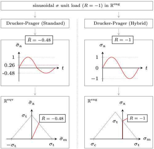
The sign of the hybrid equivalent stress is restored as the sign of the absolute largest principle stress; compare Section 6.1.
The benefit of the hybrid formulation is that it offers the choice of using the Haigh diagram in or . This is especially useful in cases where the load state is precisely known, so that interpolations and extrapolations within the respective Haigh diagram can be minimized. In this work, for instance, the Haigh diagram is more useful as this version includes data at , which is equal to the stress ratio of the biaxial tests, thus enabling a direct comparison with a single – curve.
6.3 Influences of non-proportional loads
Considering that the level of non-proportionality was found not to alter the cycles to failure for the investigated adhesive, an ideal damage prediction model will result in CFL independent of the level of non-proportionality. In this regard, the consistency of the damage prediction is more important than values close to the ideal of as a constant value might be adaptable to via calibration factors.
As mentioned in the previous section, the (signed) hybrid formulation of the Drucker–Prager criterion enables a direct comparison of the biaxial data (resulting equivalent stresses) with a single – curve (tension–compression at in ). This comparison is shown in Figure 11. Using the proposed hybrid formulation of the Drucker–Prager criterion, the resulting equivalent stress amplitude matches very well with the uniaxial – curve for the proportional load case ( °). This can be interpreted as a confirmation that equivalent stress hypotheses can be used for multiaxial fatigue analyses. However, this solely applies to the proportional load case as the predicted amplitudes do not match the – curve for the non-proportional (out-of-phase) load cases. Since the amplitude predictions of the signed hybrid Drucker–Prager criterion for the out-of-phase configurations ( °, °) are found below the – curve in Figure 11, the horizontal distance to the – curve indicates a longer fatigue life than observed by experiments as the specimens failed within the gray scatter bands.

The equivalent amplitude decline results from the phase shift in between the normal and shear stress history, because the maxima of the stress components do not overlap anymore. The decline of the equivalent amplitude with increasing phase shift is also illustrated in Figure 12 (bottom) for the signed and unsigned versions of the hybrid Drucker–Prager criterion. While the principal stress-based sign correction works fine for the proportional load case, it leads to a discontinuous time series if a phase shift and therefore a non-proportional load case is present; compare Figure 12 (black lines, bottom). Even though this discontinuous time series is not physical, it leads to significantly larger amplitudes compared to the unsigned version shown in red. In fact, the unsigned formulation rapidly gets to a level that can be considered as insignificant in terms of fatigue damage. In addition, the mean value seems to increase for the unsigned equivalent stress, which is wrong as there is no mean value in the applied axial or torsional load in the experiments.

The differences in damage prediction quality of the signed and unsigned hybrid Drucker–Prager criterion are shown at the top of Figure 12. The decrease in accumulated damage is clearly visible for an increasing phase shift for both versions and mirrors the mentioned amplitude decline. However, the signed version generates good results for (very) low phase shifts, whereas the unsigned version is significantly non-conservative at all times.
6.4 Comparison of modeling approaches
The accumulated damage of all analyzed equivalent stress formulations, Haigh diagram types, and phase shifts is shown in Table 2. Regardless of the equivalent stress formulation, Haigh diagram type, or load level, increasing levels of non-proportionality led to (rapidly) decreasing damage predictions. In a fully non-proportional case, the damage can be two orders of magnitude lower, even in case a good match was found for a proportional load case; compare in Table 2. Therefore, applications and validations of this and similar fatigue damage prediction procedures for, for example, rotor blade adhesive joints17, 20, 21 should be interpreted as solutions, which are limited to proportional load states. Hence, a more robust method such as the critical plane approach1, 2, 56-58 is required for accurate multiaxial fatigue damage predictions given that the level of non-proportionality is not zero in rotor blades of wind turbines12 and other structures. Although demonstrated with a structural adhesive, these findings can also be transferred to other materials since the root cause for the decreasing damage prediction quality is the amplitude underestimation in non-proportional cases, which is linked to equivalent stress criteria in general.
| Haigh diagram | Eqv. stress | ° | ° | ° | ° | ° | ° | ° | ° | |
|---|---|---|---|---|---|---|---|---|---|---|
| 0.210 | 0.005 | 0.000 | 0.000 | 0. 091 | 0.000 | 0.000 | 0.000 | |||
| 1.023 | 0.723 | 0.212 | 0.011 | 0.942 | 0.599 | 0.102 | 0.003 | |||
| 0.105 | 0.014 | 0.000 | 0.000 | 0.045 | 0.002 | 0.000 | 0.000 | |||
| 0.563 | 0.391 | 0.116 | 0.008 | 0.429 | 0.262 | 0.044 | 0.002 | |||
| 1.009 | 0.081 | 0.000 | 0.000 | 0.677 | 0.012 | 0.000 | 0.000 | |||
| 3.283 | 2.338 | 1.094 | 0.491 | 3.508 | 2.471 | 1.012 | 0.366 | |||
| 0.105 | 0.014 | 0.000 | 0.000 | 0.045 | 0.002 | 0.000 | 0.000 | |||
| 1.804 | 1.365 | 0.592 | 0.125 | 1.985 | 1.422 | 0.494 | 0.066 | |||
| 1.009 | 0.081 | 0.000 | 0.000 | 0.677 | 0.012 | 0.000 | 0.000 | |||
| 9.582 | 7.311 | 3.979 | 2.124 | 13.289 | 10.163 | 5.389 | 2.658 | |||
| 0.105 | 0.014 | 0.000 | 0.000 | 0.045 | 0.002 | 0.000 | 0.000 | |||
| 2.470 | 1.830 | 0.764 | 0.143 | 2.348 | 1.651 | 0.541 | 0.041 | |||
| 1.009 | 0.081 | 0.000 | 0.000 | 0.677 | 0.012 | 0.000 | 0.000 | |||
| 65.905 | 38.923 | 13.682 | 5.122 | 41.758 | 27.699 | 11.285 | 4.394 | |||
It is worth noting that all unsigned criteria predict the same damage for all Haigh diagram types in case of proportional loading ( °), for example, the von Mises criterion predicts at in each case. This is because unsigned criteria lead to a stress ratio of at °, that is, a minimum value of exactly zero; compare Figure 12 (bottom, left). This stress ratio is not affected by a tension–compression asymmetry as shown in Figures 6 and 9. Therefore, the High diagram type is not affecting the damage prediction in this case. Apart from that, even small levels of non-proportionality will lead to a drastic decrease in damage prediction quality, resulting in a very unreliable behavior of these criteria.
Based on the differences of the Haigh diagram in and shown in Figure 9, the predicted damage of signed criteria is larger when the types are used. The influences of non-proportional loads are also less pronounced in case of the Haigh diagram. For instance, the factor in between the fully proportional and fully non-proportional case using the signed Drucker-Prager criterion is 74 for the variant at and 14 for the variant.
As pointed out in Section 6.2, the difference of a hybrid version of an asymmetric yield criterion and a symmetric one is solely the shear stress sensitivity. The influence of this sensitivity can be observed by comparing the results of the signed hybrid Drucker–Prager and signed von Mises criterion in Table 2, where the latter predicts a damage that is significantly larger.
Note that the experiments did not include data at °. Therefore, the results presented above are extrapolated in this regard. However, it is expected that this represents a valid engineering approximation given the validated neutral – behavior up to °.
6.5 Discussion of modeling influences
CFL connection line types different from the piecewise linear approach will lead to different results for each equivalent stress hypothesis and phase shift. However, the general trend of a decreasing damage prediction quality with increasing levels of non-proportionality is independent of the connection line type and therefore persists.
The influence of non-proportional loads is dependent on a variety of parameters such as the load level, the ratio of normal to shear stresses and their individual stress ratio. The load level dependence is related to the decrease in equivalent amplitude with increasing non-proportionality, compare Figure 12 (bottom), and the use of the Stüssi–Haibach – approach, which introduces non-linear sections in the – diagram, compare Figure 8. The ratio of normal and shear stresses in conjunction with their individual stress ratio affects the maximum level of non-proportionality. High mean loads in combination with small amplitudes usually lead to smaller levels of maximum non-proportionality and therefore also reduce influences on the damage prediction quality. Nevertheless, non-proportional loads need to be accounted for in any case for a safe structural design.
7 CONCLUSION
Biaxial (tension/compression–torsion) fatigue tests with varying levels of non-proportionality were conducted employing a structural adhesive. It was found that non-proportional loads did not change the cycles to failure, categorizing the adhesive as a neutral material. This categorization matches recent findings where the non-proportional – behavior was connected to the ductility of a material.
An excellent specimen quality and a high number of tests increased the reliability of the results in this work, as effects of defects (pores, etc.) were negligible and the overall scatter was small.
Due to a strong tension–compression asymmetry of the investigated adhesive, implications thereof on the fatigue life prediction were analyzed. Significant differences were found comparing a Haigh diagram in the engineering and the equivalent stress space, whereat the CFL connection lines in the equivalent stress space were found below the ones from the engineering stress space. Therefore, a Haigh diagram in the equivalent stress space should be used in conjunction with equivalent stress criteria that account for a tension–compression asymmetry, for example, the Drucker–Prager criterion, to avoid non-conservative fatigue life predictions. Alternatively, a hybrid formulation of an asymmetric yield criterion allows the usage of a Haigh diagram in the engineering stress space again. This formulation was derived for the Drucker–Prager criterion in this work. As both proposals account for a tension–compression asymmetry, uncertainties with interpolations and extrapolations in the respective Haigh diagram can be minimized by choosing one of the aforementioned approaches.
An analysis of several equivalent stress criteria and Haigh diagram types was carried out concerning effects of non-proportional loads on the fatigue life prediction. The stress-based fatigue life prediction methodology resembled the state of the art in wind energy contexts. However, even in cases where a good match of the numerical prediction and experimental observation was achieved for a proportional load state, the prediction quality rapidly decreased for increasing levels of non-proportionality. As a result, fatigue life over-predictions by two orders of magnitude were found to be common for the test setup of this work. Thus, more robust methods are required to assure a reliable fatigue life prediction under non-proportional loads, which will be addressed in an upcoming publication.
AUTHOR CONTRIBUTIONS
Michael Kuhn: Conceptualization; formal analysis; methodology; software; visualization; writing—original draft preparation (lead); writing—review and editing (lead). Nikolas Manousides: Resources (µCT Scans); writing—original draft preparation (supporting); writing—review and editing (supporting). Alexandros Antoniou: Project administration; supervision; writing—original draft preparation (supporting); writing—review and editing (supporting). Claudio Balzani: Project administration; supervision; writing—original draft preparation (supporting); writing—review and editing (supporting); funding acquisition.
ACKNOWLEDGMENTS
This work was supported by the German Federal Ministry for Economic Affairs and Climate Action (BMWK) in the ReliaBlade project (Grants 0324335A and 0324335B). The authors would like to acknowledge the work of Martina Karalus and Henning Schnellen, who accompanied the fatigue experiments as technicians and implemented the machine code. Open Access funding enabled and organized by Projekt DEAL.
CONFLICT OF INTEREST STATEMENT
The authors declare no potential conflict of interests.
Open Research
DATA AVAILABILITY STATEMENT
The data that support the findings of this study are available from the corresponding author upon reasonable request.


