Enabling the Application of Graph Neural Networks on Graphs With Unknown Connectivity
Funding: This work has been co-funded by the AETHER-UA project (PID2020-112540RB-C43) funded by Spanish Ministry of Science and Innovation, and the BALLADEER (PROMETEO/2021/088) project, funded by the Conselleria de Innovación, Universidades, Ciencia y Sociedad Digital (Generalitat Valenciana). Jorge García-Carrasco holds a predoctoral contract (CIACIF/2021/454) granted by the Conselleria de Innovación, Universidades, Ciencia y Sociedad Digital (Generalitat Valenciana). This work is part of the TSI-100927-2023-6 Project, funded by the Recovery, Transformation and Resilience Plan from the European Union Next Generation through the Ministry for Digital Transformation and the Civil Service. This work has also been partially funded by the Sectorial Data Spaces projects: European Mobility (TSI-100121-2024-10) and AGROVAL-AI (TSI-100122-2024-10) funded by the Spanish State Secretariat for Digitization and Artificial Intelligence.
ABSTRACT
Graph Neural Networks (GNNs) have proven to be reliable methods for working with graph-structured data. However, it is common to find graphs with partially or fully inaccessible connectivity patterns, hindering the direct application of GNNs to the task at hand. To tackle this problem, several Graph Structure Learning (GSL) methods have been proposed, with the objective of jointly optimizing both the graph structure and the GNN model by adding loss terms that enforce desired graph properties. These properties, such as sparseness and connectivity of similar nodes, can have a drastic impact on the performance of a GNN. However, current methods offer little control on the desired degree of sparseness, which may lead to non-optimal connectivity and reduced efficiency. In this paper, we propose a new method called Adaptative Sparsification Graph Learning (ASGL), which enables fine-grained, linear control over the total number of edges in the resulting learned graph via a novel perturbation-based loss term. ASGL not only provides flexibility in sparsity control but also improves both accuracy and computational efficiency, outperforming state-of-the-art methods in most benchmarks. We demonstrate its robustness through extensive experiments and highlight how adjusting sparsity enables optimizing the trade-off between accuracy, complexity, and interpretability.
1 Introduction
There is a wide variety of data that can be naturally and efficiently expressed as graphs, such as social networks (Sen et al. 2008; Rossi and Ahmed 2015; Namata et al. 2012), traffic networks (Cui et al. 2019), 3D mesh data (Lin et al. 2021), molecular structures (X. Wang et al. 2019) or brain EEG data (Zhong et al. 2022), among others. Entities can be represented as nodes in the graph, whereas the relationship between two entities can be represented as edges connecting the different nodes.
Graph Neural Networks (GNNs) are Deep Learning (DL) architectures designed for extracting relevant patterns on graph data. Due to their representation learning capabilities, GNN models have been successfully applied to a variety of tasks, such as social network-related tasks (e.g., sentiment analysis (Y. Zhou et al. 2024)), forecasting hotel cancellations (Herrera et al. 2024), recommender systems (H. Wang et al. 2018; X. Zhang et al. 2023), emotion recognition via brain EEG signals (Zhong et al. 2022) and bioinformatics-related tasks such as drug development and discovery or the prediction of molecular properties (X.-M. Zhang et al. 2021), among others.
GNNs are particularly good at node classification tasks, that is, classifying nodes in a given graph. However, it is common to find graphs with partially or fully inaccessible connectivity patterns, hindering the direct application of GNNs to the node classification task. For example, one may have a record of previous terrorist attacks and the relationships among them stored as a graph. If, unfortunately, another attack occurs, we would not be able to directly apply a GNN for classifying the node, as the connectivity of this node remains unknown. Consequently, there has been an increasing amount of proposals revolving around the theme of Graph Structure Learning (GSL) (Zhu et al. 2021). GSL methods aim to jointly learn a proper connectivity pattern and meaningful representations for the task at hand in order to properly perform such task on graphs where the connectivity is unknown or unavailable.
GSL methods can be divided into three categories: metric learning, probabilistic modeling, and direct optimization approaches. The former ones compute the weight of an edge between two models via a distance measure between both node representations. For example, (R. Li et al. 2018) uses the Mahalanobis distance, (Yu et al. 2021) uses the inner product of the embeddings of the two nodes, (X. Wang et al. 2020) uses the cosine distance, and attentive approaches such as the GAT (Veličković et al. 2018) learn edge weights via the attention mechanism. However, these approaches can often oversimplify complex relationships by relying on fixed similarity metrics, limiting their adaptability.
The probabilistic modeling approaches are based on the assumption that the graph is generated via a sampling process and focus on modeling the probability of sampling edges with learnable parameters. For example, (Franceschi et al. 2019) model the edges by sampling from a Bernoulli distribution with learnable parameters, (Zheng et al. 2020) remove task-irrelevant edges by parameterizing the sparsification process with a neural network, and (T. Wu et al. 2020) use the attentional weights of GAT as parameters for the sampling edge distribution. Falling into this category, it is also worth mentioning Bayesian Network structure learning (Kitson et al. 2023). However, despite the flexibility of these methods, they can suffer from high computational overhead.
Finally, direct optimization approaches treat learning edge connectivities as an optimization problem, where the graph structure is learned along with the GNN. These methods include additional regularization terms in the loss function that enforce desirable properties of the graph connectivity, such as feature smoothness, sparsity, and low-rank. For example, (L. Yang et al. 2019) obtain a refined graph by including a refinement loss term based on the assumption that neighboring nodes tend to share the same label. GLNN (Gao et al. 2020) incorporates several terms to enforce properties such as sparsity and feature smoothness. Similarly, (Jin et al. 2020) includes a term for enforcing low-rank and applies it to obtain GNN models robust to adversarial attacks. Likewise, (Wan and Kokel 2021) reformulates the problem of structure learning as a meta-learning optimization problem by treating the graph structure as hyperparameters. In (W. Zhao et al. 2023), the authors successfully attempt to learn a generalizable graph structure learning model that is trained with multiple source graphs and can be directly adapted for inference on new unseen target graphs.
Despite the advances obtained so far, current direct optimization GSL methods offer little control over the degree of sparseness of the graph (i.e., the number of edges), which is one of the most important properties to take into account, as the total number of edges has a direct impact on the performance, computational cost, and complexity of the GNN model.
More specifically, current direct optimization GSL methods impose sparseness by adding a L1 regularization term on the adjacency matrix. Even though L1 regularization has been used extensively in many situations to impose sparseness, it might not be the most suitable option for GSL, because (i) it offers little to no control over the total number of edges of the learned graph and (ii) it is incompatible with learning unweighted (i.e., binary) graphs.
- We propose ASGL, a direct optimization GSL method that enables full control over the degree of sparseness of the learned graph thanks to the addition of a novel loss term based on perturbation-based interpretability methods.
- We prove the robustness of ASGL compared to the state-of-the-art via a series of node classification experiments on different datasets, where the connectivity between the nodes is fully or partially unavailable and has to be learned.
- We demonstrate that using L1 regularization to control the degree of sparseness is suboptimal. Conversely, the hyperparameter in ASGL exhibits a linear correlation with the degree of sparseness, allowing for seamless tuning and resulting in improved performance.
2 Background
In this section, we present the problem statement and the necessary background to understand our approach.
2.1 Problem Statement
Let denote an undirected graph, where , represent the different nodes and the set of connections between the different nodes. The connectivity of the graph can also be specified by the adjacency matrix , which can be binary ( if nodes and are connected, otherwise) or weighted. In this problem setup, the adjacency matrix is completely or partially unavailable, thus the connections between the different nodes are unknown.
Let each node have an associated feature vector , where is the number of features. The features of every node in the graph can be represented in a feature matrix . Moreover, the set of nodes is partially labeled, that is, some nodes have an associated label indicating its class. The objective is to predict the labels of the unlabeled nodes by exploiting the given graph information, that is, obtain a function , where contains the predicted labels for every node. This task is denoted as semi-supervised node classification.
However, the adjacency matrix (i.e., the connectivity between the nodes) is unknown, drastically increasing the difficulty of the task. Hence, the goal is to jointly obtain a node classifier while learning a proper adjacency matrix, that is, jointly optimizing both and .
2.2 Graph Convolutional Network
Convolutional Neural Networks (CNNs) have achieved impressive results when working with Euclidean, grid-like data such as images. Similarly, Graph Convolutional Networks (GCNs) are the generalization of CNNs to graph-structured data. However, the non-Euclidean nature of graphs presents several difficulties, and many approximations and variations of the convolution operation in graph data have been presented (Kipf and Welling 2017; Veličković et al. 2018; F. Wu et al. 2019; Hamilton et al. 2017).
2.3 Graph Structure Learning
As previously mentioned, direct optimization GSL methods work by jointly optimizing the GNN model and the adjacency matrix representing the connectivity of the graph. This can be done by adding regularization terms that enforce desired properties for the adjacency matrix such as feature smoothness or sparseness and imposing certain constraints such as symmetricity. A formal presentation of such regularization terms and constraints is presented below.
2.3.1 Feature Smoothness
If the th and th nodes are connected () then its features should be similar, that is, should be small in order to keep the loss term from growing quadratically larger. On the other hand, if two nodes have considerably different features, that is, is large, then it is less likely that there is a connection between them (), as the loss term would otherwise be considerable increased.
2.3.2 Sparseness
Similarly, sparseness is a topological property that can be observed across many graphs and domains (K. Zhou et al. 2013). Typically, nodes tend to form communities, where most of the nodes are only connected to a small number of neighbors.
Essentially, what this regularization term does is to encourage a fraction of the adjacency matrix values to become 1 while the rest of the values are pulled to 0. Compared to the L1 loss term, it presents the following advantages:
First, the number of edges of the learned graph is now clearly controlled by the hyperparameter , which enables experimenting with a different number of connections. Increasing the value of directly increases the complexity of the graph, which can improve the performance (or overfit, if the graph is too complex), whereas reducing simplifies the number of connection, which can reduce the performance but the resulting graph is simpler, therefore more understandable, which can be a required quality for some tasks. Second, unlike the L1 loss, it enforces the resulting graph to be binary (i.e., the connection between two nodes is either 1 or 0), which is a better approximation when working with unweighted graphs as well as it reduces the computational costs (i.e., the learned graph is simpler) and increases the interpretability of the adjacency matrix.
3 Methodology
Figure 1 shows an overview of the methodology. First, the graph learning layer receives graph node data and predicts the structure (i.e., the connection between nodes) of the graph. Then, the node information together with the learned edges are used by the graph node classifier to predict the label of every node. Finally, the ground truth labels are used to compute the loss, which will have two components, that is, the task loss and the ASGL loss, that will be used to update the weights of the graph node classifier and the adjacency matrix via backpropagation, respectively.

3.1 Graph Learning Module
3.2 Graph Node Classifier
3.3 Optimization
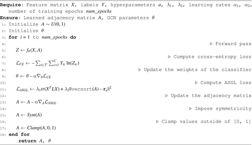
- First, a forward pass is performed and the cross-entropy loss term, , is computed.
- While keeping the adjacency matrix frozen, the parameters of the classifier are updated via backpropagation to minimize such loss term.
- Once that the parameters of the classifier have been updated, perform another forward pass and compute .
- Update the adjacency matrix via backpropagation to minimize .
In other words, the optimization procedure is separated into two steps where the cross-entropy loss is used to train the classifier, followed by updating the adjacency matrix with the ASGL loss. The total loss, which is a sum of the two terms, is only used for monitoring the improvement of the model during the training procedure. The pseudocode for this optimization procedure is shown in Algorithm 1.
Instead of using additional loss terms, there are a few other properties which can be directly imposed, therefore reducing the complexity of the problem. Specifically, we impose the adjacency matrix to be symmetric (), which essentially implies that if node is connected to node , then node is also connected to node . Enforcing symmetricity also implies that the number of learnable parameters in the adjacency matrix is reduced from to .
This is purely done for practical reasons: during training, the values of A will approach either 0 or 1 due to the sparseness term , but will never exactly reach these values due to the nature of gradient descent. Instead, the values will oscillate either around 0 or 1. By clamping the values, we reassure that the adjacency matrix is truly binary.
Figure 2 shows an illustrative example of how clamping works during the optimization. Specifically, it shows the evolution of the values of a 2 × 2 randomly initialized adjacency matrix trained via backpropagation to minimize . The experiment is performed twice, first with no clamping, and then applying clamping at every optimization step.
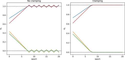
The first experiment clearly shows the previously-mentioned oscillatory behavior: initially, the values higher than 0.5 will approach 1, and the values lower than 0.5 will approach 0. As training progresses, the values will be closer to their target values. However, due to the nature of the backpropagation algorithm, there will be a point where the desired target is overshot, that is, the update rule of the values of the adjacency matrix will cause the values to be either higher than 1 or lower than 0. The following update will cause the opposite effect, therefore generating an oscillatory behavior of the values of the adjacency matrix around the target values.
On the other hand, if clamping is applied, the behavior will be exactly the same until the values overshoot its targets. When a value surpasses either 0 or 1, it will be exactly clamped to 0 or 1 respectively and therefore will not be affected by the gradients from , that is, the gradients flowing from the sparseness loss term will be zero, as the values have reached the exact target value thanks to clamping, avoiding the oscillatory behavior and obtaining a truly binary matrix.
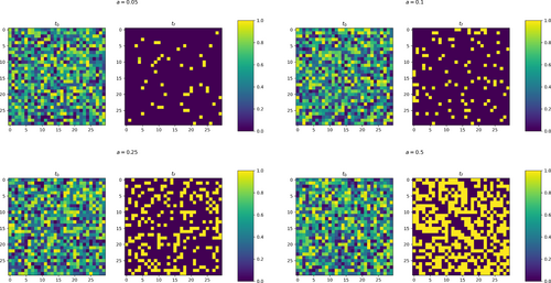
For the sake of completeness, Figure 3 shows the effect of the proposed sparseness loss on the adjacency matrix, for different values of , together with the imposed properties of symmetricity, no self-loops and clamping. As it can be seen, the resulting matrices are binary and the number of edges can be easily controlled via the parameter : for lower values of , there are less edges on the learned graph, that is, the adjacency matrix is sparse, whereas for higher values of the number of edges is higher, thus the degree of sparseness of the adjacency matrix is lower.
4 Experiments
- Compute the Euclidean distance between every pair of feature vectors, obtaining a matrix with values .
- Avoid self-loops by setting elements in the diagonal to the maximum distance
- Compute the adjacency matrix by setting an edge between the top-k closer pairs, that is, and zero otherwise, resulting in a binary, sparse adjacency matrix.
- The adjacency matrix is completely unknown; therefore, it is randomly initialized by sampling from a uniform distribution and learned during training by the GSL methods. In the baseline case, the adjacency matrix is initialized as previously mentioned and remains fixed during training.
- Information about the adjacency matrix is provided only for the training data, whereas the rest of the adjacency matrix is randomly initialized and has to be learned during training. In this scenario, an extra loss term is added to encode the available ground truth:
4.1 Datasets
We consider two citation network datasets, Citeseer (Rossi and Ahmed 2015) and Cora (Sen et al. 2008), as well as the Terrorist Attacks (B. Zhao et al. 2006) graph network dataset.
Regarding the citation networks, each dataset contains a set of scientific publications which are classified into classes according to their topic of study. Each publication is represented as a node, which contains a bag-of-words vector indicating which words in the vocabulary are present in the document. If the ith publication cites the jth, then there will be an edge between nodes and , , hence forming an undirected binary graph. Regarding the evaluation scheme, the datasets will be split into a training, validation and test split stated by (Z. Yang et al. 2016).
The Terrorist Attacks dataset consists of 1293 terrorist attacks classified according to the type of attack. Each attack is described by a feature vector containing a total of 106 distinct features. In this case, each attack will be considered as a node, whereas the edges will indicate the relation between the attacks. As this dataset is smaller than the previously-mentioned, the methods will be evaluated by performing stratified 5-fold cross validation, taking of the dataset for training, and using the remaining for evaluation purposes. Notice that the size of the training set is considerably smaller than the validation set, unlike other common Machine Learning setups. The reason behind this decision is that, given that the main advantage of ASGL is that its ability to learn the connectivity of a given graph, it is important to evaluate it on setups where the training set is relatively small, which translates to a setup where the connectivity is either fully unknown, or only a small number of connections are known.
Table 1 shows statistics for each dataset, that is, the number of documents (or nodes), the number of features per document, the number of edges, and the number of classes, as well as the number of nodes in each split (i.e., training, validation and test splits).
4.2 Implementation Details
We implemented the proposed method with the PyTorch (Paszke et al. 2019) and PyTorch Geometric (Fey and Lenssen 2019) libraries. We use two separate instances of Adam optimizers, one for the GCN and another for the adjacency matrix, both with a learning rate of . The adjacency matrix is randomly initialized from a uniform distribution between 0 and 1. In the experiments where the connectivity of the training split is given, we include such partial values into the randomly initialized . To perform a proper comparison, the adjacency matrix in the baseline case is initialized to have around of the possible connections. Similarly, the hyperparameter from GLNN is set, via trial-and-error, to obtain a similar amount of sparseness on the learned graphs. This value depends on the setup, but is typically around . One of the main advantages of ASGL is that the degree of sparseness can be controlled simply by setting . Regarding the weighting term for the feature smoothing loss, we follow the setup of GLNN and set . The input features are row normalized for numerical stability. The models were trained for a maximum of epochs with an early stopping strategy, where training stopped if validation loss did not improve after 500 epochs. The source code of the implementation will be made publicly available upon acceptance.
5 Results
Table 2 shows the results of the evaluation of the different methods on the three datasets when no information about the connectivity is provided, that is, the adjacency matrix has to be completely learned from scratch. To provide a better comparison, the experiment was repeated five times for every method and dataset, and the final result is the mean accuracy across the five repetitions. As it can be seen, ASGL obtains the best results on the Terrorist dataset, obtaining an average accuracy of . ASGL also obtains the best results on the Cora dataset, surpassing the baseline by and GLNN by . Regarding the CiteSeer dataset, ASGL obtains a lower result than GLNN, but are still comparable. As expected, the accuracies are generally low since no information about the connectivity of the graph is given and the methods have to completely learn the adjacency matrix from scratch.
| Method | Terrorist | Citeseer | Cora |
|---|---|---|---|
| GCN (Kipf and Welling 2017) | |||
| GLNN (Gao et al. 2020) | 54.68 13.56 | ||
| ASGL | 79.32 2.26 | 53.24 7.43 |
- Note: Bold values indicate the highest accuracy among all the rows within each respective table.
Table 3 shows the results of the evaluation when the adjacency matrix is partially known, that is, the edges connecting nodes on the training split are given. In this case, the baseline GCN has no improvement in terms of accuracy; in fact, the accuracy slightly decreases on the CiteSeer dataset. This behavior is expected, as there is no GSL method that enables the generalization of the structure of the training split onto the test split. On the other hand, both GLNN and ASGL have considerable improvements in accuracy for the experiments with the Citeseer and Cora datasets when compared to the previous results presented in Table 2, indicating that both methods are able to take advantage of the partial information about the connectivity of the training split. However, in the case of the Terrorist dataset, the accuracy remains similar and even decreases for the GLNN method. This is probably due to the fact that the Terrorist dataset is considerably less complex than the Citeseer and Cora datasets; therefore, it is easier for the GCN model to learn meaningful representations even though the graph structure is initialized at random, that is, GSL methods do not influence that much the resulting accuracy.
| Method | Terrorist | Citeseer | Cora |
|---|---|---|---|
| GCN (Kipf and Welling 2017) | |||
| GLNN (Gao et al. 2020) | 63.98 6.19 | ||
| ASGL | 79.00 4.23 | 67.94 3.96 |
- Note: Bold values indicate the highest accuracy among all the rows within each respective table.
In general, both ASGL and GLNN have similar mean accuracies across the experiments, but ASGL tends to have less variation on the results, that is, the standard deviation of the accuracies is lower, indicating that the results are more robust. Given that the main difference between GLNN and ASGL is the loss term controlling the sparseness, we hypothesize that, while L1 regularization encourages all values of the adjacency matrix to become small (i.e., make all edges disappear), our proposed loss term only encourages the percent of edges to disappear. We believe that this is the main cause of GLNN being less stable during training: the probability to learn a suboptimal adjacency matrix is higher, therefore leading to a lower accuracy and a higher variability across repetitions.
In addition to the increase in robustness, ASGL has a clear advantage over GLNN as it gives a clear mechanism for controlling the sparseness of the learned graph, which will be covered in the next section.
- GSL methods greatly improve the accuracy when the adjacency matrix is fully or partially unavailable, especially when the graph starts to become larger and more complex. For simpler datasets, the accuracy boost is considerable, but less drastic.
- Both ASGL and GLNN give similar results, but ASGL tends to be more stable, that is, have less variability in the accuracy across repeated experiments.
- The accuracy of ASGL increases when partial information about the adjacency matrix is provided, compared to the experiments when no information was provided and the adjacency matrix has to be fully learned from scratch. Hence, the results show that it is capable of taking advantage of such information. On simpler graphs, such as Terrorist, the increase in accuracy is negligible.
5.1 Fine-Tuning the Learned Graph Sparseness via ASGL
The degree of sparseness of the learned graph can have a great impact on the performance of the algorithm. Being able to clearly specify the degree of sparseness is desirable, as it enables the study of the tradeoff between the number of learned edges: a large number of edges can lower the performance and increase the computational cost, whereas a small number of edges can improve the interpretability of the graph but can also reduce the performance. Therefore, experiments with different degrees of sparseness are required in order to find the optimal degree of sparseness.
- In the case of ASGL, there is a one-to-one linear correlation between the hyperparameter and the percentage of edges on the learned graph. On the other hand, it is considerably more difficult to control the degree of sparseness on GLNN, as there is a small range of values of which can have impact on the sparseness. More specifically, for small values of , the percentage of edges on the learned graph is kept at a fixed value (). If keeps increasing, it reaches a point where the sparseness can be controlled, until it reaches a stagnation point, where the percentage of edges remains 0 for increasingly larger values of .
- Another important difference is that, on the case of ASGL, the degree of sparseness on the learned graph can be varied from (lowest number of edges, maximum sparseness) to (higher number of edges, minimum sparseness) of the total possible edges, whereas using the L1 loss limits the range of possible sparseness into the range
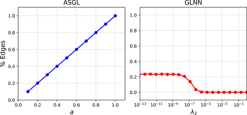
This analysis shows one of the key advantages of ASGL, which is that the degree of sparseness (i.e., the total number of edges) on the learned graph can be easily controlled, unlike L1-based alternatives such as GLNN, where the degree of sparseness is constrained into a small range which is also difficult to control. Therefore, evaluating ASGL with different values of enables finding the optimal value for the task at hand.
- If the capacity of a model is small, it might not have enough power to properly learn from the training dataset, leading to underfitting (i.e., low accuracy on validation set because the model does not have enough capacity)
- On the other hand, if the capacity of the model is too large and no regularization is applied, it will be able to learn from the training dataset so well that it will overfit to this dataset and will not be able to generalize to the validation dataset.
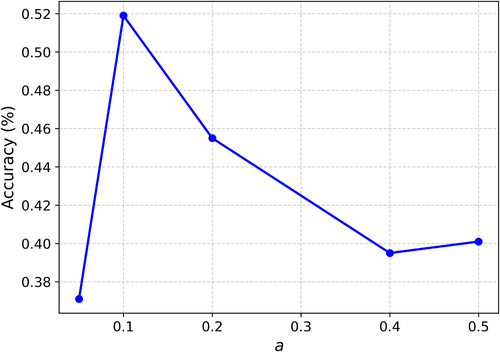
In both extremes, the resulting models are not able to properly generalize; therefore, a middle ground has to be found to obtain a proper accuracy. As shown by this experiment, the same happens with the sparseness of the adjacency matrix: A smaller number of edges (more sparse) corresponds to underfitting, whereas a larger number of edges (less sparse) corresponds to overfitting. With ASGL, the sparseness can be easily controlled so that the optimal adjacency matrix can be found.
Moreover, the sparsity of the learned graph also has an impact on the training duration. Figure 6 shows the training duration for different values of . It can clearly be seen that the time required for the same amount of epochs increases as (or the number of edges) increases. This is expected, as more edges imply more complexity in terms of message propagation.
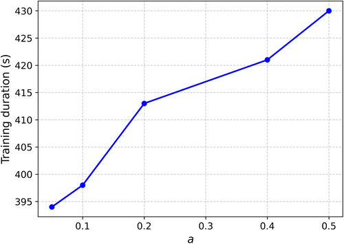
To summarize, given the results, it is clear that the degree of sparseness of the learned graph can have a considerable impact on both the accuracy and the computational cost of the model; therefore, requiring performing different trials with varying degrees of sparseness, which can be easily done by ASGL, unlike L1-based counterparts.
It is also insightful to consider the two extremes. When , the graph exhibits maximum sparsity, meaning there are no edges between nodes. This situation is akin to training a classifier to predict the class of each node based solely on its input features, as there are no edges to provide relational information. Consequently, this lack of information typically results in lower accuracy, although the computational cost of training is reduced. In contrast, when , the graph is fully connected, with every node linked to every other node. This often leads to overfitting and significantly increases the computational cost. In fact, we were unable to conduct experiments with larger values of due to excessive memory requirements.
5.2 Ablation Study
We also conducted an ablation study to quantify how each loss component of ASGL contributed to the total performance. Table 4 shows the results of the ablation study of ASGL on the Cora dataset. First, it is shown that completely removing connectivity information () causes the accuracy to drop around lower, indicating that ASGL is able to take advantage of the partially available connectivity data.
| Model | Accuracy |
|---|---|
| ASGL | |
| , | |
| , | |
| , , |
Further removing the sparseness regularizer (, ) decreases the accuracy for approximately with respect to the latter experiment. In this case, as no sparseness is enforced, the learned graph has a considerable large number of edges, which clearly impacts its performance and computational cost.
On the other hand, removing the feature smoothness term while keeping the sparseness regularizer (, ) decreases the accuracy even lower than the previous experiment. In this case, the learned graph is sparse, but the edges are randomly learned due to the fact that there is no feature smoothing term that enforces connections between similar nodes. Hence, as expected, the results are worse than in the previous experiment. Previously, even though the resulting graph had a large number of edges, some of those edges were relevant for the prediction. In this case, however, the number of edges was considerably smaller but also randomly selected.
Interestingly, removing every term (, , ) yields better results than adding just the sparseness term (, ). However, this is expected to happen, as only applying the sparseness term results in a graph with a small number of randomly learned edges. Similarly, in this experiment the edges are also randomly set, but there is no sparseness enforced, that is, the number of edges is higher, therefore more information can be propagated and the accuracy is expected to be slightly higher.
6 Conclusion
We have proposed ASGL, a direct optimization GSL method for semi-supervised node classification where the connectivity of the graph is fully or partially unavailable. By performing multiple experiments on several datasets, we have shown that ASGL achieves competitive results compared to the state-of-the-art.
Moreover, we have shown that current methods based on L1 regularization offer little to no control over the degree of sparseness of the learned graph structure, whereas ASGL enables full control via a hyperparameter , which is linearly correlated to the percentage of edges on the learned graph.
This work provides both theoretical and practical insights into controlling the degree of sparseness in graph learning. From a theoretical perspective, our approach offers a more principled mechanism for sparsity control compared to conventional L1 regularization. While L1 regularization is commonly used to enforce sparsity, it has inherent limitations in range control, as it saturates at a certain point and does not allow fine-grained manipulation of the number of edges. In contrast, our method enables precise and linear control over the sparsity level through a dedicated hyperparameter, providing greater flexibility and interpretability in graph structure learning. From a practical standpoint, the ability to adjust the density of the learned graph is highly desirable for real-world applications, where different domains exhibit varying levels of connectivity. Some problems require highly dense graphs to capture intricate relationships, while others benefit from sparser structures for improved efficiency and generalization. By allowing explicit control over graph density, our method empowers practitioners to tailor the learned graph structure to the specific needs of their applications, striking a balance between computational cost, model interpretability, and predictive performance.
We also show that being able to properly fine-tune the degree of sparseness of the learned graph can considerably improve performance, as well as allow studying the trade-off between the number of edges: as shown by the performed experiments, too many edges can lower the performance as well as increase the computational cost; a smaller amount of edges reduces the computational cost and is easier to interpret, but performance may also decrease. Hence, being able to properly control the degree of sparseness enables finding the optimal result.
Despite the advantages and improvements of ASGL, it is also important to acknowledge its limitations. One limitation is its applicability to highly dynamic graphs, where the structure changes frequently over time. In such scenarios, ASGL may struggle to adapt quickly to evolving connectivity patterns, potentially leading to suboptimal performance. However, it is important to remark that dynamic graph structure learning remains an open challenge (Z. L. Li et al. 2023). Additionally, given that ASGL has a loss term that encourages that similar nodes should be connected, it is susceptible to noisy feature data. However, it is important to remark that these limitations were already present in previous direct optimization approaches to GSL.
Future work will be directed towards solving these challenges. Specifically, we will explore adaptive mechanisms for dynamic graphs, such as online or incremental learning, to enhance the applicability of ASGL in evolving network structures. Additionally, we aim to investigate robustness to noisy features and the integration of ASGL with other GNN architectures, such as Graph Attention Networks, to improve performance across diverse real-world applications. Another key focus will be on optimizing the joint learning process of both the node classifier and the adjacency matrix. Currently, the two-step optimization scheme can cause the adjacency matrix to converge rapidly, limiting the information flow between the learned graph structure and the classifier. Addressing this limitation will be crucial in refining the ability of ASGL to generalize and adapt to complex graph scenarios.
Acknowledgments
This work has been co-funded by the AETHER-UA project (PID2020-112540RB-C43) funded by the Spanish Ministry of Science and Innovation, and the BALLADEER (PROMETEO/2021/088) project, funded by the Conselleria de Innovación, Universidades, Ciencia y Sociedad Digital (Generalitat Valenciana). Jorge García-Carrasco holds a predoctoral contract (CIACIF/2021/454) granted by the Conselleria de Innovación, Universidades, Ciencia y Sociedad Digital (Generalitat Valenciana). This work is part of the TSI-100927-2023-6 Project, funded by the Recovery, Transformation, and Resilience Plan from the European Union Next Generation through the Ministry for Digital Transformation and the Civil Service.
Conflicts of Interest
The authors declare no conflicts of interest.
Open Research
Data Availability Statement
The data that support the findings of this study are openly available in GitHub at https://github.com/jgcarrasco/asgl.


