A social interaction model with an extreme order statistic

1. INTRODUCTION

There is a growing body of literature in which the influence of social peers in economics and other social sciences is addressed; see Durlauf (2004) for a recent survey. Conventional social interaction models, including the spatial autoregressive model and the linear-in-means model, assume that an individual's outcome depends linearly on the mean of the outcomes of the individual's peers; see, e.g. Anselin (1988), Manski (1993), Moffitt (2001), Lee (2007) and Bramoulle et al. (2009). For instance, a student's test score would be affected linearly by the mean test score of their classmates. In certain situations, we believe that a better specified model might involve the full distribution or other distributional characteristics, such as order statistics, rather than the mean (e.g. Ioannides and Soetevent, 2007).

In this paper, we introduce a social interaction econometric model with an extreme order statistic to allow non-linearity in modelling endogenous peer effects.1 Let be a finite set of players in a social network (group) and let be the set of players, except the ith player, who are i's neighbours. For example, a simple social interaction model with the maximum statistic for the ith player is specified as , where denotes and is a random element. The social interaction model with the minimum statistic can be defined in a similar way.

Empirical studies have found evidence regarding peer effects on educational outcomes; see, e.g. Hanushek (1992), Hanushek et al. (2003) and Hoxby (2000). It is plausible that peers affect educational outcomes by aiding learning through questions and answers or by hindering learning through disruptive behaviour. Lazear (2001) has suggested that disruptive students could interfere with the educational outcomes of their peers. For instance, a student who has bad grades in class might hinder learning by asking poor questions. This disruptive behaviour might have large negative effects on the academic achievements of this student's peers, and thus might generate strong endogenous peer effects. Figlio (2007) has found empirical evidence of the effects of disruptive students on the performance of their peers, which indicates that students suffer academically from the presence of classroom disruption. Thus, our social interaction model with an extreme order statistic might be useful to explore such ‘bad apple’ effects in some empirical studies.

In many real-world situations, rewards are based on relative performance rather than absolute performance, and competition in terms of extreme outcomes may occur. Holmstrom (1982) has suggested that a relative performance scheme provides a better evaluation than an absolute performance scheme in the presence of costly monitoring of the agent's effort. Lazear and Rosen (1981) have suggested that there is a convex relation between pay and performance level in tournament schemes.2 Frank and Cook (1995) have attributed much of this phenomenon to winner-take-all markets, which compete fiercely for the best. Examples of such schemes include companies offering bonuses to the ‘salesperson of the year’, universities rewarding researchers for writing the ‘best paper’ and athletes being rewarded for having the best Olympic performances. Main et al. (1993) have conducted a detailed survey of executive compensations and have found some support for a relative performance scheme. Ehrenberg and Bognanno (1990a,b) have found that the performances of professional golf players are influenced by the level and structure of prizes in major golf tournaments.

In contrast to the situation where individuals are competitors in the labor market, individuals can benefit from their peers in a social group. The benefit might take the form of the sharing of know-how between individuals. This is an efficient way for individuals to obtain valuable experiences from their peers and especially from those who are most capable.3 Therefore, individuals might react to the performance of their best peers in a strategic model of social network.

The paper is organized as follows. In Section 2., we provide some theoretical justifications for the social interaction model with the minimum or maximum statistic on economic grounds. In Section 3., we introduce a general model specification with an extreme order statistic. We show that the social interaction model with an extreme order statistic is a well-defined system of equations. The solution to the system exists and is unique. Our model has the essential features of a static game with complete information for a finite number of players. In particular, this game is asymmetric and has a unique pure-strategy Nash equilibrium. In Section 4., we provide a simple instrumental variables (IV) approach for a general model where exogenous regressors are relevant. In Section 5., we consider the generalized method of moments (GMM), which uses IV moments and recurrence relations for moments of order statistics. Our asymptotic analysis of estimation methods (IV and GMM) is based on a sample consisting of a large number of groups where group sizes remain fixed and bounded (as the number of groups tends to infinity). In Section 6., we give a brief introduction of an extended social interaction model with mixed mean and maximum. In Section 7., we provide some Monte Carlo results and in Section 8., we provide an empirical example. To illustrate the practical use of this model, we apply it to the National Collegiate Athletic Association (NCAA) men's basketball data and we obtain some interesting results. In Section 9., we draw our conclusions. In Appendix A, we list some useful notations and some moments of ordered normal random variables. In Appendix B, we give detailed proofs of the theorems provided in Sections 3., 4. and 6.. In Appendix C, we provide a brief description of the maximum likelihood estimation (MLE) of simple model specifications and some Monte Carlo results. In Appendix D, we give a useful lemma and some technical details about the GMM estimation with recurrence moments discussed in Section 5..

2. THEORETICAL ECONOMIC CONSIDERATIONS

Our model specification can be derived from a simultaneous move game with perfect information.4 The sample can be viewed as repetitions of a game played among individuals with possibly varying finite numbers of players. We give three theoretical examples to illustrate the model specification within the game-theoretic framework. These theoretical models are for illustrative purposes and are not exclusive for possible economic applications of the proposed econometric model.

2.1. A synergistic relationship

A game has m players involved in a synergistic relationship (Osborne, 2004). It is a static game with complete information, in which each player knows the pay-offs and strategies available to other players. Each player's set of actions is the set of performance levels. Denote by a performance profile chosen by players and by , which is a subvector of p with dimension , the performance profile of all players except the ith player in the game. Player i's preference is represented by the pay-off function , which depends on p in the following way. First, and capture the concave relationship between pay-offs and performance levels. Secondly, , , captures the synergistic relationship between player i and player i's peer j.

For analytical simplicity, assume that each player is endowed with one unit of social capital (i.e. for all i). The social capital can only be used to establish social connections between players. If player i spends an amount on j, then player i's pay-off can increase proportionally by . Intuitively, the player will spend all their social capital in establishing connections with their peers such that . Formally, we have the pay-off function

(2.1)

with . Note that represents the cost of performance, which is similar to the moral cost in the crime network study of Liu et al. (2011). It should be stressed that , which is a function of characteristics of the individual i, varies across individuals. In other words, 2.1 depends on which player chooses the action. So, the game is asymmetric. To maximize the pay-off, the player will spend all their capital on their best peer who has the highest performance level in the synergistic relationship.5 So, we have that

(2.2)

Suppose that each player chooses the optimal performance level to maximize (2.2), which gives the reaction function of player i as

(2.3)

where the coefficient ϕ is non-negative. For empirical estimation, we expect that , the performance profile, is observable, and the index will be specified as , where is a vector of observed characteristics of individual i and represents the characteristics that are unobservable by econometricians. Here, ϕ and β are unknown parameters for estimation.

As an alternative specification, it is possible to justify the game in terms of choosing effort instead of performance level directly, as long as the response of an individual to their peers is on their maximum performance level. Suppose that an individual chooses their effort to respond to the best performance of their peers. Then, we have . Suppose that the performance of individual i is the sum of their effort and unobserved disturbance (i.e. ). Then, the model with the measurement relation becomes , which is similar to 2.3, where is the overall disturbance.

2.2. A tournament scheme

In a tournament game, we assume that a player is rewarded based on relative performance. We assume that the gross pay-off depends on p in the following way. First, and capture the convex relationship between pay and performance. Secondly, reflects the competition among players (Calvo-Armengol and Zenou, 2004). Formally, we have the gross pay-off function in a tournament game

(2.4)

where varies across individuals. With , player i will be rewarded for winning the tournament, and penalized for losing. Suppose that player i's cost is a convex function of performance with and . Formally,

(2.5)

Combining all the above information, the net pay-off can be written as

(2.6)

Each player will do their work in order to maximize the net pay-off according to the first-order condition

(2.7)

The second-order condition requires , which is sufficient for a maximum at . It follows that the reaction function is

(2.8)

where the coefficient of is negative. For estimation, and would be functions of the observable and unobserved characteristics of individual i by econometricians. Here, ρ and ϱ would be unknown parameters. Because and would also involve unknown coefficients of individual characteristics, only the composite parameter can be identifiable in this model if only are observed but not the costs .

2.3. A game that combines the tournament scheme and the synergistic relationship

In the above example, the cost function (2.5) can be written as

(2.9)

which captures the benefits of social interactions between connected players (Calvo-Armengol and Zenou, 2004). To achieve the most benefit, a player will allocate all their social capital to the best peer in order to minimize the cost. So, we have that

(2.10)

We obtain the net pay-off function

(2.11)

which gives the best response function

(2.12)

Note that the coefficients of in (2.3) and (2.8) are positive and negative, respectively. We can interpret the former as the social effect and the latter as the competition effect. The net pay-off function (2.11) combines the tournament scheme and the synergistic relation into a single game. In this situation, the coefficient of in (2.12 ) would represent the difference between the social effect and the competition effect, so that it can take either a negative or a positive value. Its sign indicates the domination of one effect over the other. They cannot be separately identified from (2.12) alone. These effects would be separately identified if the cost or pay-off of a player could be observed. In the next section, we shall see that the best response function (2.3), (2.8) or (2.12) has a unique Nash equilibrium under some general conditions.

3. THE SOCIAL INTERACTION MODEL WITH MAXIMUM AND REGRESSORS

The various reaction functions on the performance of a player with respect to the maximum performance of their peers in Section 2. are just examples. In order to provide a general model and its estimation, we consider a model specification with the outcome of an individual being and the outcome profile of the individual's peers being . The individual's observed characteristics will be represented by a vector of regressors and unobserved characteristics involved will be summarized as . So, in general, we consider the social interaction model with maximum and regressors:

(3.1)

Here, m is the total number of players in a game, is a vector of observed individual characteristics and is an individual disturbance, which is known to the agent but unobservable to econometricians. Thus, the reaction functions 2.3, 2.8 and 2.12 can all be included in this framework. For example, λ will be for 2.12, and will become in this general formulation. Because and possibly vary across individuals, 3.1 can be interpreted as the reaction function for an asymmetric game with perfect information. With given individual characteristics and , 3.1 can have a unique Nash equilibrium when . The following theorem summarizes the solution of 3.1 as the unique Nash equilibrium.

Theorem 3.1.Denote for simplicity. The system 3.1 with but is equivalent to the following system with order statistics:

(3.2)

Here, and are the corresponding order statistics of and in ascending order. The system 3.2 has the unique solution:

(3.3)

Analogously, for the social interaction model with minimum, , the solution exists and is unique as and for given but . We note that the existence and uniqueness of the solution are valid without any distributional assumption on .

We see that, from the arguments of the proof for Theorem 3.1, as long as but , the order statistics have the same ascending order as . In this case, the solution (Nash equilibrium) of the system exists and is unique. The restriction provides the stability of the system. However, the system is unstable or divergent when .

It is apparent that the system has many possible solutions when λ is 1 or −1. This is also the case with . For any , consider the quantities defined by , and with but . The quantities of these elements have the order . They also imply and . When , ; hence, these for satisfy the structure and form a solution set. For , because i can be any individual of , there are multiple solutions for the system.

For certain estimation methods, such as the method of maximum likelihood (ML), a unique solution of the system is essential, because it requires a well-defined mapping of the disturbance vector to the sample vector conditional on observed exogenous variables in order to set up the likelihood function. However, for certain estimation methods, such as IV or the two-stage least-squares (2SLS) estimation, even though the system might have multiple solutions, asymptotic analysis of such estimation methods could still be valid as long as proper instrumental variables are available for the endogenous explanatory variables of the structural equation and the rank condition is satisfied, under the scenario that the number of groups R tends to infinity but the group sizes remain finite and bounded.6

The social interaction model with an extreme order statistic can be compared with the group interaction model based on the average outcome of peers,

(3.4)

with . This group interaction model allows individuals to interact with each other within a group, and peer effects are reciprocal in the model. The social interaction model in 3.2 implicitly assumes that every player except the best player depends on the first-order statistic (i.e. the group maximum). There are no reciprocal effects between players except for the first- and second-order statistics in 3.2. The conventional group interaction model is a special case of spatial autoregressive models, which assume exogenous interaction structures. In contrast, the interaction structure of the model with an extreme order statistic is endogenously determined. It resembles an extension of a star network but the star is endogenously determined with the adjacency matrix of the form7

4. ESTIMATION

Suppose that the economy has a well-defined group structure. Each player belongs to a social group. The players can interact with each other within a group but not with members in another group. The sample consists of R groups with players in the rth group. The total sample size is . For empirical relevance, we allow variable group sizes in the model but group sizes remain finite and bounded as the number of groups increases.8

For the estimation, we make the distinction whether exogenous regressors are present or not in the model. Because the model with exogenous regressors might be more relevant for practical use, we focus on the estimation of this general case in the main text, whereas the estimation of the model without regressors is given in Appendix C.

4.1 The model with exogenous regressors

The model 3.1 can include observed group factors as well as individual characteristics :

(4.1)

Here, and denote and vectors of exogenous variables. If and are relevant regressors, the IV approach is possible and is distribution-free.

Assumption 4.2. are i.i.d. random variables with zero mean and a finite variance , and are independent of and .

With , in terms of order statistics in Theorem 3.1, the system 4.1 is equivalent to

(4.2)

where and are the transformed variables of x and ε, respectively, under the permutation of y into an ascending order. The and are not necessarily in ascending order, even though .

With and being constants, are independent but not identically distributed, so the likelihood function for can be complicated. Under normality, the density of conditional on and is , where is the standard normal density function. Conditional on and , the joint density of the order statistics is

(4.3)

where the summation S extends over all permutations of (David, 1981, p. 22). The density function for is

(4.4)

Because the possible number of permutations is large in general, the ML approach will be computationally demanding unless the number of players in a game is very small. Furthermore, a parametric ML approach will not be distribution-free. For tractable estimation, we consider an IV approach.

Because and are exogenous, important moment restrictions of 4.1 are , and for all . The number of such IV moments is . In order to distinguish possible parameter values from those of the true values that generate the sample observations, a subscript 0 on parameters is added to indicate their true values. Because and , the model via (4.2) implies that

(4.5)

with . Because ,

(4.6)

Similarly,

(4.7)

and

(4.8)

Similar to , can also have

(4.9)

Denote and for or 3. Then, , which has zero mean by mutual independence of x and ε. It follows that provides a set of valid instruments,

(4.10)

as long as does not collapse into any of its lower-order power variables for .9

Denote and Writing 4.1 in vector form, we have

(4.11)

where , , and are the corresponding vectors and matrices in the rth group, is the -dimensional vector consisting of ones in its entries, collects all these explanatory variables in a single matrix and δ₁ is the complete vector of coefficients. Let be a generic IV matrix for , which satisfies the following assumption.

Assumption 4.3.The probability limits of and exist and are non-singular. Furthermore, 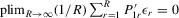and

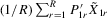Assumption 4.3 requires that has full rank asymptotically, which is a sufficient condition for the identification of δ₁. The IV estimator with for 4.11 is

(4.12)

Theorem 4.1.Under Assumptions 4.1–4.3, the IV estimator with is consistent and

Let denote a matrix consisting of , , , and some powers of .10 The 2SLS estimator with 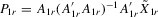is

(4.13)

with the asymptotic variance . For the estimation of σ², the moment 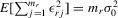implies that a variance estimator can be

(4.14)

4.2. The model with exogenous regressors and group effects

The model 4.1 can be extended to include an unobservable group factor

(4.15)

which is equivalent to

(4.16)

and

For generality, we allow to correlate with or . Hence, it is desirable to treat as fixed effects. However, there is a need to eliminate the incidental parameter's problem as R tends to infinity, for which purpose, we consider the deviation from a group mean operation. Denote , and , where , and are the corresponding group means. Pre-multiplying 4.16 by the transformation matrix , individual observations are measured as deviations from group means

(4.17)

and

with .

Because are exogenous, important moments of 4.15 are for all . By multiplying each equation in 4.17 by the corresponding , , and taking their summation, the model via 4.17 implies that

because . Hence,

(4.18)

Note that any constant regressors within the group will not be useful for the within-group equation because the summation over all units of 4.17 in a group is identically zero. For IV estimation, additional instruments are needed for on the right-hand side of 4.17. Denote for or 3. Because , which has zero mean,

(4.19)

Denote . The within-group equation of 4.15 is

(4.20)

where , , , and are the corresponding vectors and matrices in the rth group. Let be a generic IV matrix for , which satisfies the following assumption.

Assumption 4.4.The probability limits of and exist and are non-singular. Furthermore, and

Assumption 4.4 requires that has full rank asymptotically, which is a sufficient condition for the identification of δ₂. The IV estimator with for 4.20 is

(4.21)

Theorem 4.2.Under Assumptions 4.1, 4.2 and 4.4, the IV estimator with is consistent and

Let denote a matrix consisting of and some of its powers. The 2SLS estimator with is

(4.22)

where its asymptotic variance is . For the estimation of σ², the moment implies that a variance estimator can be

(4.23)

5. THE GMM APPROACH

If all the exogenous regressors were irrelevant, the above IV methods would no longer be applicable. In other words, if β₀ and γ₀ were zero, IV moments alone would not identify the model parameters. Furthermore, it is impossible to test the joint significance of all the exogenous regressors based on those IV estimators. To remedy such a possible but unknown scenario, we suggest a combination of IV moments with some recurrence relations for moments of order statistics. The resulting estimation method is distribution-free. However, when regressors are really relevant, the validity of the recurrence relations would require that the regressors are i.i.d. for all i and r, which is a strong assumption of this estimation strategy for the model.

We consider the GMM approach for the general model, namely 4.15. Denote , which has the same ascending order as in terms of order statistics. We can eliminate the common group effect of 4.15 by the differencing method, and we obtain the following system

(5.1)

and

(5.2)

Assumption 5.1. and are i.i.d. for all members in a group as well as across groups.

Recurrence relations for moments of order statistics are based on the i.i.d. property of random variables. Let and be the ith-order statistics in random samples of size m and , respectively. We have a useful recurrence relation

(5.3)

which follows directly from a lemma of Balakrishnan and Sultan (1998) in Appendix D. Denote for . Equation 5.3 implies

(5.4)

for . By taking , 5.4 implies that

(5.5)

for . Denote and for . For a generic group of size m, the system of equations 5.1 and 5.2 implies that

(5.6)

for , and

(5.7)

for . It follows that and for . The corresponding moment in terms of dependent variables of 5.1 and 5.2 is

(5.8)

for . As in the general GMM estimation framework, let be some weighting matrix such that is non-negative definite. The GMM estimator with weights is , which minimizes , where is an empirical moment vector consisting of the recurrence moment 5.8 and the IV moments for the model 4.15. The GMM estimator satisfies the first-order condition

Assumption 5.2. converges in probability to a constant weighting matrix a₀ with a rank no less than , and converges in probability to D₀ that exists and is finite.

Theorem 5.1.Under Assumptions 4.1, 4.2, 4.4, 5.1 and 5.2,

where .

By the generalized Schwartz inequality, the optimal choice of a₀ is . It follows that the optimal GMM estimator minimizes , where is a consistent estimate of V₂ (see Appendix D for details on the Proof of Theorem 5.1).

6. THE MODEL WITH MIXED MEAN AND MAXIMUM

We consider a generalized social interaction model with mixed mean and maximum as follows,

(6.1)

with , or, equivalently,

(6.2)

Following Theorem 3.1, 6.1 with but is a well-defined system and has a unique solution. It includes the social interaction with the mean or maximum of peers as a special case. For empirical application, we provide a simple IV estimator under the fixed-effects specification.

Denote . As , it implies that and . The within-group equation of 6.1 is

Writing the within-group equation of 6.1 in vector form, we have

(6.3)

where collects all explanatory variables in a single matrix, and is the corresponding parameter vector. Let be a generic IV matrix for , which satisfies the following assumptions.

Assumption 6.1.Assume that for all r where the lower bound and the upper bound m_U are finite. Furthermore, either or there are sufficient number of groups with .

Assumption 6.2.The probability limits of and exist and are non-singular. Furthermore, and

Assumption 6.1 requires that group sizes are not all less than three for model identification, because and are identical for . Assumption 6.2 requires that has full rank asymptotically, which is a sufficient condition for the identification of δ₃. The IV estimator with for 6.3 is

(6.4)

Theorem 6.1.Under Assumptions 4.1, 4.2 and 6.2, the IV estimator with is consistent and

Following Lee (2007), we can use as an IV for . Let denote a matrix consisting of and in 4.22. The 2SLS estimator with is

(6.5)

with the asymptotic variance . Similarly to 4.23, the variance estimator of is

(6.6)

7. MONTE CARLO RESULTS

The models used to generate are given by 4.1 and 4.15, and these are

We randomly draw from the standardized χ²(5) distribution to investigate finite sample properties of distribution-free estimators under this non-normal distribution. The two regressors and are i.i.d. N(0, 1) for all r and i, and are independent of . The group effect is generated as . The true parameters are , , and . We allow group sizes to vary from three to five. We design the same number of groups for each group size. The average group size is four by design. In the simulation, we experiment with different numbers of groups R from 60 to 1920. The number of Monte Carlo repetitions is 300.

We try two different IV estimators. IV1 uses the group average of 4.9 as instruments, and IV2 uses and of 4.10 in the first model. Because is invariant within the group, only IV2 is relevant to the second model. We also consider the GMM and the two-step procedure (TSP). The GMM uses IV1 and recurrence relation 5.3 for the first model, and uses IV2 and 5.8 for the second model. For computational simplicity, we use the identity matrix as a weighting matrix in a GMM objective function.11 The TSP uses the moments of 5.3 or 5.8 to estimate λ in the first step, and then regresses fitted residuals on exogenous variables to estimate their coefficients by the ordinary least-squares method in the second step.

Table 1 presents the bias (Bias) and standard deviation (SD) of IV1, IV2, GMM and TSP estimates of Model 1. The IV1 and IV2 estimates of λ are unbiased for all R. The GMM estimate of λ is biased upward when or 120, and this bias decreases as R increases. The TSP estimate of λ has a large upward or downward bias when or 120, but this bias decreases sharply when or more. All the estimates of λ have smaller SDs as R increases. The IV1 estimate of λ has much smaller SDs than those of the other estimates. The IV2 estimate of λ has larger SDs than those of the GMM estimates for all R, and has smaller SDs than that of the TSP estimate when or less. However, it has larger SDs than that of the TSP estimate when or more. These estimates of β, γ, μ and σ have similar properties in bias and standard deviation. Table 2 presents finite sample results of IV2, GMM and TSP estimates of Model 2. The IV2 estimate of λ is unbiased for all R. The GMM estimate of λ is biased downward when or less, and this bias decreases as R increases. The TSP estimate of λ has large upward bias when or 120, but this bias decreases sharply when or more. The GMM estimate of λ has smaller SDs than those of the IV2 and TSP estimates. These estimates of β and σ have similar properties in bias and standard deviation.

If exogenous regressors are irrelevant to the model, the IV method is inconsistent. However, GMM and TSP, which use recurrence relations for moments of order statistics, remain valid. For illustration, we present finite sample results of the IV, GMM and TSP estimates of the models when β₀ and γ₀ are zero. The IV1 estimate of λ has significant upward or downward bias for all R in Table 3, and the IV2 estimate of λ has significant downward bias for all R in Table 4. In contrast, the GMM and TSP estimates of λ have smaller biases and these biases decrease as the number of groups increases.

8. AN EMPIRICAL EXAMPLE

In college basketball, all major individual player awards are given based on regular season performance. For example, the John R. Wooden Award is given to the most outstanding college basketball players every year. For the winners of these awards, it is not only a great honour, but it also increases the probability of being drafted by a National Basketball Association (NBA) team, which has the highest average salary among major sports leagues. In our example, we assume that a college basketball player i in a team r will maximize his net pay-off function 2.11. After the reparametrization of 2.12, we obtain his best response function:

(8.1)

Note that and capture observed and unobserved common group factors (e.g. coach effects), respectively, which are eliminated by the covariance transformation in our fixed-effects estimation framework. As a comparison, we estimate the group interaction model with the mean specification as well as the generalized model 6.1.

There are over 10,000 men's basketball players competing in three divisions at about 1,000 colleges and universities within the NCAA. Division I (D-I) has the most prestigious basketball programmes, which have the greatest financial resources and attract the most athletically talented students. We collect men's basketball player statistics of D-I teams during the period 2005–2010 from web sites including ncaa.org, espn.com and statsheet.com. The total number of teams (groups) is 1,673 in the five seasons.12 The total number of observations is 22,122. The average team size is 13, with a minimum of eight and a maximum of 20.

Table 5 reports the descriptive statistics of variables used in the regression analysis. We measure per-game performances of a player, based on his various accomplishments, such as points, assists, rebounds, steals and blocks. These accomplishments are the most important factors in determining his chance of winning the awards and/or becoming an NBA player. Our measures are different from the player efficiency rating (PER), which measures a player's per-minute performance.13 Some experts have criticized the PER on the grounds that it gives undue weight to a player's contribution in limited minutes. Hence, we use the per-game performance to measure a player's contribution to the team. We use several per-game performance measures () as the dependent variables of our regression models. There are five measures that are different combinations of points, assists, rebounds, blocks and steals. Estimated results of each of these are reported separately in Tables 6–10. Specifically, we have the following measures for the dependent variable for a player:

1. the dependent variable in Table 6 is the points per game of a player;
2. the dependent variable in Table 7 is the sum of points and assists per game;
3. the dependent variable in Table 8 is the sum of points, assists and rebounds per game;
4. the dependent variable in Table 9 is the sum of points, assists, rebounds, and steals per game;
5. the dependent variable in Table 10 is the sum of points, assists, rebounds, steals and blocks per game.

The explanatory variables for each of the Tables 6–10 are the same, and include height, weight and minutes per game. Height gives a major advantage in professional basketball, because taller players generally achieve more rebounds, block more shots and make more dunks than shorter players. Weight might also give a college player some advantages, because strength is an important factor in many aspects of the game. Both height and weight will have a positive effect on a player's performance. Minutes per game is defined as the total minutes played in one season divided by the number of games played, and this is expected to have a positive coefficient. For reasons of scale, we divide weight and minutes per game by ten in the actual regressions.

Tables 6–10 report the regression estimates under the fixed-effects specification. Column (1) presents the within-group IV estimates of 6.1, for which there are no endogenous interaction regressors. We find that the coefficients of these regressors (i.e. the elements of the vector discussed above) are statistically significant. Physical characteristics (with an exception in Table 7) have positive estimates, which indicate that taller and stronger athletes play better basketball. Table 7 uses the sum of points and assists as the performance measure, and finds that height has a negative effect. The point guard is one of the most important positions on a basketball team, and players at this position are shorter and are awarded more assists, which might explain the unexpected sign of height. Minutes per game is potentially endogenous because coaches generally give better players more time on the court. Hence, we use the years of college education (freshman, sophomore and junior) as the instruments for this endogenous regressor, and the IV estimates are statistically significant and positive.

Because interaction regressors are endogenous, we use the instruments proposed in Section 4.2 for the best performance of peers and the instruments proposed by Lee (2007) for the average performance of peers. Columns (2) and (3) show that the interaction regressor has a negative and statistically significant effect in the respective model.14 Column (4) shows that both interaction regressors remain negative in the generalized model 6.1. The best performance of peers is statistically significant, whereas the average performance of peers is statistically insignificant, except for the case that uses the sum of points and assists as a performance measure. Column (5) presents the GMM estimates of the model 8.1, which are similar to the IV estimates.15 We conclude that a college basketball player reacts negatively and statistically significantly to the best performance of his teammates, which suggests that there exist important competition effects among basketball players in an NCAA D-I team.

9. CONCLUSION

In this paper, we introduce a social interaction econometric model with an extreme order statistic, which differs from conventional social interaction models in that an individual's outcome is affected by the extreme outcome of peers. Our model represents one of the possible extensions to allow non-linearity in modelling endogenous social peer effects.

We show that the social interaction model with an extreme order statistic is a well-defined system of equations. The solution to the system exists and can be unique. We provide a simple IV method for model estimation if exogenous regressors are relevant. A distribution-free method that uses recurrence relations is applicable, even when regressors might be irrelevant. It should be noted that ML estimation would be infeasible for the model including exogenous regressors (unless the number of players is very small), even if one were willing to make a distributional assumption of the disturbances, because the likelihood function of order statistics for independent but not identically distributed variates is rather complicated.

We apply the social interaction models with peer's maximum, peer's average and a mixed specification to the NCAA D-I men's basketball data. We find that a college player performs negatively and statistically significantly in response to the best performance of his peers, which suggests the existence of competition effects in the basketball game. For future research, we can apply this model to explore the possible ‘bad apple’ effect in an empirical study of education. We can also consider a model with reaction to certain quantiles of the outcome distribution.