
Geodesic Distance Computation via Virtual Source Propagation
Abstract
We present a highly practical, efficient, and versatile approach for computing approximate geodesic distances. The method is designed to operate on triangle meshes and a set of point sources on the surface. We also show extensions for all kinds of geometric input including inconsistent triangle soups and point clouds, as well as other source types, such as lines. The algorithm is based on the propagation of virtual sources and hence easy to implement. We extensively evaluate our method on about 10000 meshes taken from the Thingi10k and the Tet Meshing in the Wild data sets. Our approach clearly outperforms previous approximate methods in terms of runtime efficiency and accuracy. Through careful implementation and cache optimization, we achieve runtimes comparable to other elementary mesh operations (e.g. smoothing, curvature estimation) such that geodesic distances become a “first-class citizen” in the toolbox of geometric operations. Our method can be parallelized and we observe up to 6× speed-up on the CPU and 20× on the GPU. We present a number of mesh processing tasks easily implemented on the basis of fast geodesic distances. The source code of our method is provided as a C++ library under the MIT license.
1. Introduction
Geodesic distance is the generalization of Euclidean distance to manifold domains and, as such, it is the natural metric for geometric constellations on meshes. This makes it a fundamental tool in geometry processing and important for many techniques such as remeshing [PC06], shape descriptors [IAP∗08,GBK16,TBIpS11], shape interpolation [SdGP∗15], animations [WLCJ12], deep learning on geometry [BMM∗15, MBBV15], and many more.

Figure 1: Single-source-all-destination approximate geodesics computed by our method, Geodesic Source Propagation (GSP), on a large mesh with complex topology. Exact geodesic iso-contours are shown in sharp red lines and ours as color gradients in dark blue to avoid occlusion. Source is the red sphere. On a single 4.5 GHz core, our method can process about 4–10 million vertices per second. Speed and accuracy (as mean relative error) are representative of what our method achieves on the Tet Meshing in the Wild [HZG∗18] data set.
Computing exact geodesic distances on meshes turns out to be impossible in linear or quasi-linear time because the distance function itself is only piecewise analytic—empirically with 풪(|V|1.5) pieces and 풪(|V|2) in the worst case [SSK∗05, MMP87].
Thus, a lot of research went into fast but accurate approximations. While most of the exact algorithms are based on window propagation [SSK∗05, CH90], approximation algorithms take many forms: from graph-based Dijkstra-style or fast marching solutions of the Eikonal equation, to the heat method which is based on a connection between geodesic paths and physical heat propagation.
For practical applications, exact methods are often too slow and the approximation algorithms all come with trade-offs or limitations such as expensive or memory-intensive pre-computation, parameter fine-tuning, or strong requirements on mesh tessellation quality. This makes it hard to choose any particular algorithm without knowing the exact use case. To be considered a first-class citizen in the standard toolbox of geometric processing, an algorithm for geodesic distances should practically run in linear or quasi-linear time, have low and predictable approximation error, be usable in an unsupervised setting, and be versatile enough to be used as a sub-component of other algorithms. These are the criteria that we aim to improve and that guide the structure of this paper. Through careful analysis we developed a conceptually simple but thoughtfully assembled method.
Many methods for approximate geodesics, such as fast marching [NK02] or DGPC [MR12], propagate per-vertex distance values. When a new vertex distance is computed, previous distances are used to reconstruct a virtual geodesic source from which the new distance can be derived. In Section 3.1 we argue that this only works well if the mesh is roughly convex and isotropic. Otherwise, the previous distances may not refer to the same virtual source resulting in a poor reconstruction, jeopardizing following computations. We solve this by propagating an explicit representation of the virtual source instead of reconstructing it on-the-fly. An efficient representation and update step is presented in Section 4.1.
A central component of most Dijkstra-based algorithms is a priority queue. From a performance point of view, such a queue is suboptimal in theory due to its 풪(|V| log |V|) complexity and in practice due to multiple indirect memory access and bad cache locality. It is also notoriously hard to parallelize, especially on the GPU. In Section 4.2 we present an efficient alternative using two FIFO queues that we call a dual queue system. These queues can be processed independently, within certain limits, allowing a parallel implementation.
In Section 4.3 we show that with a sufficiently fast update step the layout of the mesh in memory now becomes a bottleneck due to cache misses. Hence, we provide a simple topological bottom-up clustering algorithm that significantly improves cache locality.
1.1. Contribution
Our Geodesic Source Propagation (GSP) is a propagation-style approximation algorithm for geodesic distances on triangular meshes.
-
To improve accuracy, we propagate virtual geodesic sources instead of just scalar distance values.
-
To improve performance, we replace the priority queue by a dual queue system based on two FIFO queues, formulate the algorithm in an intrinsic parametrization, and optimize the memory layout.
-
The explicitly propagated virtual sources improve robustness.
-
Being an iterative propagation at core and having access to richer information provides significant flexibility and versatility.
-
Our dual queue system enables an efficient parallel implementation with up to 6× speed-up on the CPU and 20× on the GPU.
To demonstrate that we achieve these goals, we evaluate our method on about 10000 meshes taken from real-world data sets representing both low and high quality input. We show that our method is faster than state-of-the-art algorithms for approximate geodesic distances—even faster than the pre-factorized heat method. At the same time, our algorithm only produces a fraction of the error of second-order fast marching or the heat method, especially for challenging tessellations. With no precomputation required, it is now possible to compute single-source-all-destination geodesic distances as fast as other elementary mesh operations.
In this paper we present the fundamental concepts and ideas of our method. More details on the implementation, additional evaluation, and a C++ implementation under MIT license is provided at https://graphics.rwth-aachen.de/geodesic-source-propagation.
2. Related Work
2.1. Window Propagation
Most algorithms based on window propagation can be traced back to the work of [MMP87], called the MMP algorithm. The original work turned out to be too complex to implement with the first practical version of this algorithm proposed and implemented by [SSK∗05], sometimes known as the SU algorithm. Their algorithm also supports approximative geodesics by merging windows during the update step. [BK07] extends Surazhsky's window propagation from point to polygonal sources. An alternative class of algorithms was started by [CH90] known as the CH algorithm, later improved by [XW09].
Many papers focused on improving the performance of window propagation style algorithms. [XWL∗15] use a bucket queue to be able to process many windows in parallel, resulting in the FWP-MMP and FWP-CH algorithms. [YXH14] propose a parallel version of the CH algorithm, PCH. A GPU version of the CH algorithm was developed by [YHF∗19]. By cleverly culling redundant windows, VTP [QHY∗16] is currently one of the fastest exact geodesics algorithm. Even with all the improvements, window propagation algorithms remain slow, memory demanding, and difficult to implement robustly.
2.2. Partial Differential Equations
The classical approach to generating distance functions is to find a function φ: Ω → ℝ satisfying the eikonal equation |∇φ| = 1, as well as φ(x) = 0 for all source points x ∊ S ⊂ Ω. One of the most popular class of methods for solving this equation is fast marching [KS98]. The original update step computes a linear approximation of the distance function. [NK02] raise the approximation quality to second order while [TWZZ07] improve the handling of boundaries. Fast marching also works on incomplete data, point clouds, and in volumetric scenarios [MS01,MS05,CK11].
Instead of trying to solve the non-linear hyperbolic eikonal equation, the heat method [CWW13] solves a linear elliptic partial differential equation for heat transport. This leads to a very efficient algorithm that requires solving one diffusion and one Poisson equation which can both be pre-factorized per mesh. [BF15] provides several improvements and alternative algorithms for geodesic distances based on PDEs. Finally, [SSC18] extend the heat method to vector fields while also making the original formulation more robust by utilizing an intrinsic Delaunay triangulation. A parallel version of the heat method was proposed by [TZD∗18].
For meshes that can be partitioned into a few grid-like domains, [WDB∗08] propose an efficient, parallel fast marching on the GPU. Using similar domain decomposition techniques, [KCP∗16] were able to achieve significant speedups. While showing substantial speedups, their dependence on domain decomposition limits their applicability.
2.3. Precomputed Graphs
Another interesting trend is to compute a graph structure in an expensive pre-processing step. Using this graph, subsequent queries can be answered efficiently and with high accuracy. While the precomputation makes them unsuited for dynamic data or infrequent queries, they shine if the mesh is static and many queries must be answered.
The GTU method [XYH12] precomputes a sparse geodesic triangulation and a large lookup table to answer approximate geodesic in 풪(1) time per query. The Saddle Vertex Graph (SVG) [YWH13] is a sparse undirected graph containing an edge for every pair of saddle vertices that are connected by a straight geodesic path. This graph can be constructed in an incomplete fashion to obtain an approximate but faster solution. A similar idea is the Discrete Geodesic Graph (DGG) [WFW∗17]. Instead of using saddle vertices, the DGG can use arbitrary points as relays.
2.4. Other
[CR87] show that the construction of exact geodesic paths in three dimensions is NP hard. Their construction relies on extremely small differences in paths and thus does not rule out existence of efficient approximation algorithms. [MVC04] provide an iterative scheme to improve approximate geodesic paths by use of the straightest geodesic theory. For anisotropic geodesic distances, [CHK13] develop a so called short-term vector-valued Dijkstra.
Local texture coordinates for meshes can be computed via geodesics as well. [SGW06] approximate a discrete exponential map by propagating a single source vector over edges. Their approach is only used locally and never introduces new virtual sources, effectively only computing completely straight geodesics. DGPC [MR12] computes polar coordinates using a propagation with an update step similar to fast marching with the improvement by [TWZZ07]. They additionally propagate an angle in order to reconstruct texture coordinates.
3. Method
3.1. Virtual Geodesic Sources
The core intuition for our method is shown in Figure 2. Geodesic paths are piecewise straight lines [MMP87]. When viewed on the unfolded path from target to source, we even get a stronger guarantee where tangent discontinuities, “corners”, can occur: at boundary vertices with angle sum above 180° or interior vertices with angle sum over 360°, i.e. saddle vertices.

Geodesic paths on triangle meshes consist of piecewise linear segments when unfolding the triangles from target to source. Tangent discontinuities, “corners”, can only occur at boundary vertices with angle sum above 180° or interior vertices with angle sum over 360°, i.e. saddle vertices. Top shows the convex case, bottom the saddle vertex case. In both cases, the unfolded triangles are shown dashed with a transparent blue filling. The geodesic path is shown in solid red on the mesh and dashed red on the unfolded triangles. Corners also act as “virtual sources”, which we exploit in order to propagate accurate, yet compact information over the mesh.
These virtual (geodesic) sources are the central piece of information that our method propagates over the mesh. Instead of computing complete geodesic paths, we only need to propagate the virtual sources s and the length of geodesic path that is “behind the corner”, σ. In the unfolded domain from target to source, this virtual source is the first corner on the geodesic path and the rest of the path length is stored in σ. Thus, the geodesic distance from target t to source is simply |t – s| + σ, given that t and s are represented in the same unfolded space, e.g. in the tangent space of the triangle containing t as shown in Figure 2 (bottom).

Window propagation algorithms that compute exact geodesics propagate these virtual sources with extra distance σ. However, one virtual source per triangle is insufficient in general and many might be required. Thus, the exact algorithms typically store a variable number of such sources on edges, enough information to reconstruct exact distances to vertices.
On the other side of the spectrum, approximation algorithms often only propagate scalar distance values, incurring a heavy loss in information. A simple Dijkstra using edge lengths can be considered the most trivial geodesic approximation algorithm. Creative update rules have been proposed that try to locally reconstruct as much information as possible in order to increase the accuracy. The most accurate of these are fast marching using the update step from [NK02] with extension from [TWZZ07] and DGPC [MR12]. Given two vertex distances in a triangle, they try to find a virtual source s that satisfies these distance constraints in the supporting plane of this triangle. Using this virtual source they compute the distance to the third vertex and apply a heuristic when the geodesic path should bend and get a new corner.
There are two obvious sources for inaccuracies: the reconstruction and the bending heuristic. Reconstructing s from two vertex distances is not possible in general. Even if the two distances are exact, they might already contain extra distances σ before the last corner. In that case, the radius for the radial reconstruction is not the complete distance, but only a part of that. Without explicit tracking, it is impossible to know what radius to use. The two vertex distances could also belong to different virtual sources, for example behind a saddle vertex or if multiple geodesic fronts meet. And finally, as soon as even one distance becomes inaccurate, the reconstruction cannot recover.
The bending heuristic determines whether the update uses a straight geodesic or if a new corner should be introduced. Fast marching with Novotni's update step never bends. The third vertex is always computed assuming the path to the reconstructed source is straight. Tang's extension to fast marching and DGPC, on the other hand, bend if the quad formed by the triangle and the virtual source is non-convex. This is equivalent to testing if the line from the third vertex to the source intersects the gate edge e.
Our method, called GSP, avoids the first problem by propagating an explicit representation of the virtual source s, including the extra distance σ as a separate value. Instead of propagating over vertices, we propagate from triangle to triangle. A triangle has a well defined tangent space in which we can express the virtual source s. The bending—in contrast to the reconstruction—cannot be made fully accurate as that would require storing and processing a variable number of virtual sources per triangle. However, we can refine the heuristic.
3.2. Data-Driven Visibility Heuristic
The propagation of geodesic distances from triangle D to a point p in triangle E across the common edge e is only valid if the line of sight from p to the virtual source s (in tangent space) crosses the edge e. Since the visibility status of s can vary for different positions of p in E, exact geodesic distance computation requires the storage of multiple sources (“windows”) for each triangle. To reduce complexity and increase efficiency, approximate geodesic distance computation relies on storing just one virtual source per triangle and hence may over- or under-estimate the true distance depending on the local mesh configuration. Propagation algorithms for approximate geodesics differ in the heuristic they apply to determine source visibility.
The inset shows that perfect accuracy cannot be achieved: the two meshes have the same triangles D and E. Only considering the triangle E and previously computed geodesic paths from D, it is impossible to determine what virtual source to store in E. If a new virtual source is introduced at v, G will use that new source and q‘s geodesic would be (q, v, s), which is too long. On the other hand, if no new source is introduced, F will also point to s and p‘s geodesic ends up being (p, s), which is too short. This simple example demonstrates that the correct source information for propagation cannot be predicted from triangles D and E.

A conservative choice is to test source visibility with respect to the corner in triangle E, opposite to e. If the source is visible from the opposite corner, it is visible from any other point in E (i.e. the quad spanned by E and s is convex). This heuristic is conservative since it introduces a new virtual source as soon as s is not visible from some point in E. As a consequence geodesic distances tend to be over-estimated. In our algorithm described so far, we use the center of gravity c for the visibility heuristic which is a balance between over- and under-estimation because some points in E lie above and some below the line of sight from the center of gravity to the virtual source. For irregular triangulations, however, this heuristic can also cause significant approximation errors. Instead of deriving more sophisticated heuristics, we determine one in a data-driven fashion.
Let c be the center of gravity of triangle E and a the opposite corner to triangle D. Then we check virtual source visibility for a point b = λ · c + (1 – λ) · a between c and a. The point b acts as a kind of visibility probe. The blending weight λ is derived as a function of some anisotropy measures on E.

More concretely, we compute the following four anisotropy measures for the triangle E given its edge lengths ei (shared edge is e1) and height h of triangle E on e1:

By comparing them to four thresholds  , we obtain a four-bit binary signature (i.e. 16 possible patterns). Via a small look-up table we get the blending weight λ. This procedure has 20 parameters (4 thresholds plus 16 look-up table entries) which are optimized once via a simple genetic optimization algorithm and then kept fixed for all meshes. Using this data-driven heuristic instead of always using the center c (λ = 1) or the opposite corner a (λ = 0) leads to an observed reduction of the average approximation error by about 20% in our experiments. The setup for training this function and the exact parameters can be found in the supplemental material.
While more complex heuristics might lead to better approximation errors, they also tend to be more expensive to evaluate. Our heuristic might seem arbitrary, but it does not increase the runtime noticeably and is motivated by the fact that mesh anisotropy correlates strongly with approximation error (Figure 9). In general, the problem is not curvature-related anisotropy, but slivers and thin triangles caused by modeling tools, e.g. due to decimation, hole filling, or fan-based polygon triangulation. All geodesic paths through triangles must be represented by a single virtual source and this assumption is empirically violated for thin and long triangles more often than for regular ones. The relative error is typically largest in the neighborhood of these anisotropic triangles. We conjecture that this is also the reason why our training on a few meshes nevertheless generalizes well: The anisotropy measures τi roughly summarize the (very) local neighborhood in a scale-independent manner. Training on a small subset of meshes then still means that we optimize over a large variety of local neighborhood scenarios as long as the meshes are sufficiently diverse. We leave a full investigation into ideal trainings setups and more general but still efficient heuristics to future work.
3.3. Propagation
Our algorithm starts by constructing the virtual source information explicitly for all triangles that are adjacent to the real sources. For sources inside a triangle only the triangle itself is initialized, for sources on vertices all neighboring triangles are initialized. In both cases σ = 0 and s is set to the tangent-space vector from the triangle center to the source. All halfedges from the initialized triangles are added to a queue. A halfedge represents the edge that we want to propagate over but also indicates which triangle is source and which is target.
Until the queue is empty, we take enqueued halfedges and compute a new virtual source for the target triangle using the propagation rules depicted in Figure 3. If the geodesic distance to the center using the new source is lower than what the target triangle had previously stored, we update the information in the target triangle and enqueue its two remaining neighboring halfedges. The propagation can potentially update triangles multiple times and from different incoming edges.

Propagation of virtual geodesic sources over triangle edges. When propagating from one triangle into a neighboring one, both triangles are unfolded over the shared edge (green) into a common tangent space first. The virtual source s of the first triangle can now be used in the second triangle. If the line from the second triangle's heuristic point (here visualized as the center) to the virtual source does not intersect the shared edge, a new virtual source is created at the closest edge vertex v and the additional distance σ′ = |s – v| is added to the previous extra distance σ (step 3).
This is similar to a label-correcting algorithm such as [Ber93]. Which type of queue we use has little effect on the result because all triangles are updated until they contain the shortest geodesic path. The traversal order mainly affects the runtime of the algorithm. An obvious choice would be to use a priority queue using center distances as key, which would make this a Dijkstra-type algorithm. In Section 4.2 we show how using two FIFO queues results in an algorithm that is significantly faster in practice. Convergence of our propagation is guaranteed because only shorter paths trigger additional updates.
The actual step of propagating the information (s0, σ0) of the source triangle t0 into the target triangle t1 over the halfedge h is:
-
Convert s0 from t0‘s tangent space to t1‘s by unfolding both triangles along their shared halfedge h into a common plane. The result is s1.
-
Test if h intersects the line from t1's heuristic point to s1 (cf. Section 3.2).
-
If yes, (s1, σ0) is the new virtual source for t1.
-
If no, use (v,σ0 + |v – s1|) where the new virtual source v is the vertex of h closest to the old virtual source s1.
Step (3) and (4) will only override the previous information if the distance to the center is shorter. Notice that (4) can overestimate the true geodesic distance but in this case it will be overwritten later, when the propagation scheme reaches this triangle via another halfedge. Under-estimation can also happen if s1 is not actually visible from the complete shared edge. Visibility is only checked with local information, but could be blocked later on the unfolded path. This is more serious because it cannot be corrected later. The test in (2) ensures that the geodesic path of the target triangle actually goes through the source triangle and is key to maintaining accuracy. If not for this test, all geodesics would be considered straight and impossible paths would compromise accuracy as can be seen in Figure 3 (step 3). Algorithm 1 lists the full procedure. Note that this is only a conceptual description of how the propagation works. Section 4.1 describes a way to perform this update step efficiently using an intrinsic parametrization.
4. Algorithm Design
The previous section introduced our method on a conceptual level. We complement this by discussing the necessary steps to implement our approach in an efficient and robust manner. In particular, Section 4.1 presents how the virtual source update step can be made fast and robust by using an intrinsic parametrization. Section 4.2 presents our dual queue propagation scheme based on two FIFO queues that is easy to implement and more efficient than a priority queue. In Section 4.3 we highlight the importance of (and present solutions to) traversing the mesh in a cache coherent manner. Finally, Section 5.7 discusses parallel implementations on the CPU and GPU.
4.1. Efficient and Robust Parametrization
In Section 3.3, the information that is propagated per triangle T is (sT, σT) where sT is a 2D vector living in the tangent space of the triangle pointing to the previous geodesic event, i.e. a virtual or real source. σT is a scalar tracking the additional distance from the virtual source to the original one.
The update step, propagating over edges, requires expressing the adjacent triangles in a common coordinate system and even with pre-computation and optimizing operations, this causes non-negligible cost. However, the change of coordinate system is not required if the algorithm operates purely on an intrinsic parametrization of the mesh. In this parametrization, the input are not 3D vertex positions but edge lengths ei. s is not propagated as a vector but instead each vertex v of a triangle T stores the distance dv,T to s. Because vertex-triangle pairs (v, T) can be identified with halfedges, we store dv,T per halfedge. σT is still stored per triangle and we additionally store dT, the geodesic distance of the triangle center in order to simplify the test whether the propagated distance is shorter than the previously stored one. In the actual implementation we store  instead of dv,T to save a few operations. Thus, per triangle the 5-tuple
 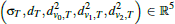 is stored. This parametrization is similar to the window propagation of [SSK∗05] and a logical evolution of [TWZZ07]'s update step.
ALGORITHM 1: Geodesic Source Propagation (GSP)
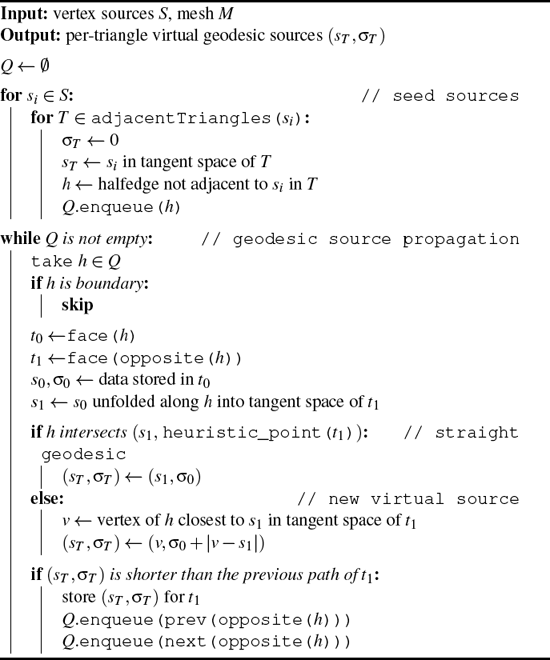 |
To demonstrate the simplicity of the formulas and provide a reference for implementation, the update step is given in full detail. The inset shows static (black), given (red), and computed (green) variables. We are free to choose a local coordinate system, so we place the edge that we are propagating through on the x axis with vertex A being at the origin.

The propagation happens over the halfedge h, from the previous triangle U into the current triangle T. At the beginning of the update step we know the values  and
and  , representing the distance to the virtual source S, and σU, denoting the additional distance to the real source. We want to compute all required values for the current triangle T.
Given edge lengths e1, e2, and e3 we can reconstruct the third triangle point P via

The virtual source S is reconstructed with a similar formula:

Py and Sy have different signs because they lie on opposite sides of h. The barycenter C of the triangle is easily found with

At this point, the heuristic of Section 3.2 is invoked and returns a new point Q that should be used to test visibility. (The previous inset shows the case Q = C.) The x coordinate of the intersection between  and
and  , called t, can be computed via linear interpolation:

We can now distinguish three cases:
-
if t < 0, there is no intersection and the source is in negative x direction. A is the new virtual source, resulting in:

-
if t > e1, there is no intersection and the source is in positive x direction. B is the new virtual source, resulting in:

-
there is an intersection and the virtual source stays the same:

Additionally, there is the case that the virtual source and triangle lie on the same side of h, which can happen in situations as depicted in step 3 of Figure 3 (step 2 still uses the original source and propagates that over the last halfedge in step 3. From that perspective, the original source is on the same side as the triangle center and we always introduce a virtual source at a vertex.) In this case we will never have an intersection of  and
and  . Instead we directly compute two lengths:

l1 corresponds to the length of the path from S to C over A while l2 corresponds to the length of the path from S to C over B. If l1 is shorter, we use case (1), otherwise case (2).
In the end, a new triangle distance d′T is computed. If it is smaller than the previously stored one, we replace the values dT, σT,  ,
,  , and
, and  . The propagation continues by enqueuing h2 and h3. At this point we can compute the 2D normals n2 and n3 (of the edges e2 and e3):

Using the sign of the dot products (S – A)T n2 and (S – B)T n3, we can check if the virtual source S lies on the same side of h2 or h3. This one bit of additional data is also propagated in the queue and used in the update steps for h2 and h3 to check which case we are in.
4.2. Dual Queue Propagation
Section 3.3 outlined the basic propagation and suggested that Dijkstra-style priority queues might not be the best choice when optimizing for performance. A priority queue, even cleverly implemented, has logarithmic complexity, multiple memory accesses per look-up, and bad cache behavior. Instead, we employ two FIFO queues 풜 and ℬ in a dual queue scheme:
-
initialize 풜
-
while 풜 is not empty:
-
for all entries e in 풜:
-
if skip-condition, add e to ℬ,
-
otherwise compute update step for e
-
and enqueue new entries in 풜 or ℬ (based on queue-policy)
-
-
start next iteration by setting 풜 ← ℬ and ℬ ← 0
-
Entries are enqueued in step (iii) only if a new shortest path is found, making this a label-correcting instead of label-setting method. Additionally, entries are skipped if they became stale, i.e. if a shorter path for them was enqueued. Depending on skip-condition and queue-policy we can formulate different propagation strategies:
-
By never skipping and always enqueuing in ℬ we recover the classical breadth-first search, effectively expanding in order of topological distance. Because there is typically a mismatch between topological and geodesic distance, many duplicate expansion steps and label corrections must be performed.
-
For the speed limiter strategy we never skip but enqueue in 풜 if the geodesic distance dT is smaller than f · i and in ℬ otherwise. This roughly causes all triangles up to f · i distance to be expanded in the i-th iteration and delaying expansion of triangles “further away”.
-
In the postpone strategy, new entries are always enqueued in ℬ but we skip the update step (postpone the entry) if dT > di for some per-iteration fixed maximal distance di. In static postpone we choose di = f · i. Dynamic postpone sets di = minprev dT + f using the minimum geodesic distance of the previous iteration. As a middle ground, hybrid postpone uses di = max (minprev dT + f0, di–1 + f1). The postpone strategies are feasible because skipping entries is a lot cheaper than duplicated updates. In the limit f = ∊, they mimic the behavior of a priority queue because the next expansion would always be the next bigger dT.
f, f0, and f1 are global parameters, i is the index of the current iteration. These strategies differ in the average number of enqueue and update operations and how well they adapt to anisotropic meshes. In addition to the propagation strategy, there is the choice to store 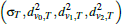 either in the mesh (lean queue) or in the queue entries (fat queue).
In our extensive experiments, we found that for a single-threaded implementation, speed limiter with f = 1 and a lean queue works best. In a parallel setting (cf. Section 5.7), speed limiter is problematic because the size of 풜 changes during execution and the lean queue requires a critical section when updating the per-triangle tuple. There, we found that hybrid postpone with f0 = 1, f1 = 0.1 and a fat queue works best. As the same halfedge can be in the queue multiple times, the lean queue approach saves memory bandwidth. However, it requires more elaborate locking in the parallel case (the update of all values must be atomic), which is why the fat queue is preferable there (only dT requires an atomic update). For a similar reason, the postpone strategies are a good fit for parallel implementations. As already stated, speed limiter uses concurrent modification of the queue that is iterated over, which interferes with parallel scheduling. In contrast, the postpone variants embrace the “ping-pong” strategy that is typical for parallel implementations. One “wave” of jobs is scheduled for processing 풜 and the result is written to ℬ. Then, the roles of 풜 and ℬ are swapped. The “Parallel Implementation” Section of the supplemental material contains more details. The inset shows the single-threaded performance of these strategies on a few isotropic and anisotropic meshes. Shaded region is standard deviation. Note that the edge lengths are normalized such that f = 1 corresponds to the average edge length.

The main advantage of the dual queue schemes is that they have little overhead and are simple to implement. They exploit the inherent regularity in mesh graphs which is strongest for isotropic meshes. This is reminiscent of the bucket queue used in [XWL∗15] but simpler (while still being effective). For meshes with roughly uniform triangle size, our algorithm empirically runs in linear time. The intuition behind this is that each iteration updates a certain “geodesic distance band”. For roughly regular triangulations, the number of times a triangle can be updated before the next “band” is reached tends to be bounded. Even when this uniformity constraint is not satisfied, the simplicity of this dual queue approach beats the priority queue in most cases. In Section 5.3 we evaluate real-world performance of this approach on a big data set consisting of meshes of both types, including stress tests with highly non-uniform meshes. The dual queue approach is applicable to many Dijkstra-style algorithms, especially if the actual update step is simple or if a label-correcting approach must be used anyways. The inset shows the number of times a triangle's value was updated on a challenging mesh. The source is on the cat's right ear.

In the worst case, the strategies degenerate (at least locally) to the breadth-first search (BFS) and expand in topological instead of geodesic order. This can for example happen if f for the static postpone strategy is chosen so large that nothing is postponed in practice. Dynamic postpone has a large execution time if the mesh has areas with dense and coarse triangulations. The whole front is slowing down if parts of it touch the dense region (as the di is increased only slowly). We observe linear time for roughly regular triangulations. However, even for the Thingi10k meshes, we encountered only locally quadratic growth, mainly around abnormally large or long triangle triangles.
4.3. Cache Coherent Mesh Layout
With the update step and dual queue propagation scheme presented in the last sections, the cost of propagation is now dominated by memory access. In general, we cannot expect the order of vertices, faces, and halfedges to be optimized for algorithms that traverse the mesh in an unpredictable manner. In our experience, meshes usually have a recognizable memory layout. Some result from isosurface extraction or laser scans where the line-by-line processing is still visible. Others, like incremental decimation, tend towards random layouts. Different cache layouts with memory index coded as hue are shown in the inset.

With the above optimizations applied, the computational cost of a propagation step is only about 100 CPU cycles. However, taking memory access into account, it can increase this to over 800 cycles on bad layouts.
Optimizing the layout of a graph for random walk traversal, or even specifically the layout of a mesh are well-researched topics. See for example [YLPM05] or [YL06]. For high quality layouts refer to those papers. Nevertheless, we want to briefly present a very simple and fast algorithm for optimizing mesh layouts that proved to be sufficient in our tests to significantly reduce the cost-per-update-step, even for bigger meshes. This is closely related to fill-in reduction strategies [CM69,KK98].
Figure 4 shows the effect of different memory layouts on our algorithm. We used a grid mesh of different sizes to compare several “natural” layouts. The seed vertex is the center of the grid.
-
rows. Line-by-line layout. Traversing in one direction is cache-friendly, the other is always a miss.
-
random. Shuffled layout. Every traversal is a cache miss.
-
BFS. Breadth-first order starting from the seed vertex. While entries in the current queue tend to be cache-friendly, other neighbors are usually not in the same cache line.
-
Z. Z-order curve fractal. This layout is only defined for power-of-two grid sizes but has the property that neighbors in all directions tend to be close in memory.
-
optimized. Our simple but effective layout optimization via bottom-up clustering.

Cost of GSP on different memory layouts across different sizes measured in cycles per update step. Standard deviation over multiple runs is shown shaded. The test mesh is a grid. See Section 4.3 for a description of the different layouts. Our layout algorithm performs as well as the Z-order curve, which is only well defined for power-of-two grid sizes. Note that in all cases the executed instructions are the same. The only difference is the memory layout.
For small meshes that can be kept completely in the L1 or L2 cache, layout does not matter much. However, for large meshes the effect can be drastic. Almost random layouts can incur up to 700% overhead. Semi-structured layouts such as “rows” or “BFS” still have 150–200% overhead. Only optimized layouts such as the Z-order curve or our approach can bring the overhead down to about 50%.
The idea of our layout optimization is a simple greedy bottom-up clustering approach. A cluster consists of vertices and initially each vertex is in its own cluster. Clusters are progressively merged, resulting in a tree of merge operations. Traversing the tree leaves in-order produces the final memory layout. Child order did not matter much in our tests.
We perform the clustering in iterations as depicted in Figure 5. Each iteration has a vertex limit that grows exponentially: the first iteration has a maximum cluster size of 1, the second of 2, the third of 4, and so on. In each iteration we greedily merge pairs of clusters if the result obeys the vertex limit. Merge attempts are ordered by the number of mesh edges connecting two clusters. Pairs of clusters with many edges between the clusters are merged first. The intuition here is that in order to keep cache misses low, neighboring vertices should get similar indices in memory. The earlier two clusters are merged, the more similar their indices become. To avoid an 풪(|V|2) algorithm, pairs of clusters should be considered only if they have connected vertices.

Simple but effective bottom-up clustering scheme for optimizing cache layouts: In iteration i, sets of vertices (black) are merged unless the result exceeds 2i vertices. Order of merging is determined by number of original mesh edges between two clusters (red), in descending order. An in-order traversal of the leaf nodes of the resulting tree gives a cache layout that considerably reduces cache misses for mesh-traversal type algorithms.
To implement this approach efficiently we recommend using a union-find data structure [TvL84] as each iteration produces a disjoint partitioning of the vertices. In our evaluation, the layout optimization only took a few milliseconds per mesh on average.
The effect of cache optimization on various geodesics algorithms can be seen in Table 1. Note that this optimization is purely topological and does not consider positions or edge lengths. Geometric information is not required because propagation-based algorithms expand the topological neighborhood of their propagated primitives and we optimized the probability that, given a primitive, its direct neighborhood is nearby in memory. As a side remark, our optimization also benefits the heat method because sparse matrices derived from cache-optimized meshes tend to have less fill-in.
| method | original | optimized | random |
|---|---|---|---|
| Dijkstra (priority queue) | 43 ms | 34ms | 110 ms |
| Dijkstra (dual queue) | 20 ms | 13 ms | 66 ms |
| VTP | 1940 ms | 1836ms | 2278 ms |
| Heat Method (Eigen) | 73 ms | 69 ms | 227 ms |
| Heat Method (CHOLMOD) | 216 ms | 119 ms | 322 ms |
| FMM | 275 ms | 240 ms | 372 ms |
| DGPC | 275 ms | 263 ms | 387 ms |
| GSP (ours) | 56 ms | 38 ms | 160 ms |
4.4. Other Extensions
As a propagation-style algorithm, extending and customizing the update step is rather simple. Some examples for such extensions are custom source types, anisotropic metrics, and unstructured domains (shown in Figure 6). The explicitly propagated virtual source information can be used to increase reconstruction accuracy (Figure 7). More details can be found in the supplemental material.

Our method can be extended easily. The update step can be formulated to include other primitive types, such as lines (a). The intrinsic parametrization makes anisotropic metrics almost trivial (b). Using k nearest neighbor queries, geodesics on point clouds can be computed (c).

Geodesic distances for a tessellated cube. The source is on the back side. (b) shows linear interpolation of vertex distances. In (c), the per-triangle virtual source is used to compute the distances. The transition between different virtual sources can be refined by also considering neighboring triangles (d). Exact result is shown in (e).
5. Evaluation
Evaluation was done on a 4.20 GHz Intel Core i7-7700K (4.5 GHz single core turbo) with 16 GB RAM and an NVidia GeForce RTX 2080. Except if otherwise noted, all computations were performed on a single CPU thread, time was measured using the rdtsc instruction which measures CPU cycles. Using cycles as the measurement unit makes the results better comparable across different CPUs and clock rates. It also mitigates inaccuracies caused by the turbo mode, which dynamically changes the CPU frequency. All algorithms were implemented in C++, compiled with Clang 7 using the flags -O3, -march=native, and -ffast-math.
5.1. Methods
Dijkstra is implemented using an std::priority_queue. For GSP on point clouds domains we used the nanoflann library [BR14] and 10 neighbors per propagation step.
Our implementation of the heat method uses the Simplicial-LLT solver from Eigen [GJ∗10] and the Supernodal solver from SuiteSparse [CDHR08], both with double precision sparse matrices. Note that contrary to our method, 64 bit precision is required. Cotangent weights are part of the precomputation step and do not contribute to the solve part of the heat method. Fine tuning of the time step t was not possible due to the number of evaluated meshes. As suggested in [CWW13], we uniformly used t = 1.0 · h2 where h is the average edge length. An intrinsic Delaunay triangulation as suggested in [SSC18] was not used as this is another costly preprocessing step and has its own problems with malign meshes.
To the best of our knowledge, there is no reference implementation for fast marching, so we used our own that is reasonably optimized and includes triangle unfolding to deal with obtuse meshes. We compare different update steps: the original gradient update step from [KS98], the radial update step from [NK02], and the improvement on Novotni's update from [TWZZ07]. The implementation of the Local Vector Dijkstra is kindly provided by [CHK13]. [MR12] published a reference implementation for DGPC. For evaluating accuracy, we use the VTP window propagation [QHY∗16] to obtain the ground truth.
5.2. Evaluation Data Set
Accuracy and performance strongly depends on the mesh and source. Memory layout is seldom accounted for. For a robust comparison, we chose to evaluate on the Thingi10K data set [ZJ16] consisting of real-world meshes used in 3D printing. These are mostly generated from CAD programs and include highly anisotropic meshes as well as wildly varying triangle sizes. Many triangles are degenerate and many meshes are non-manifold. For geometry processing, this is a malign data set. [HZG∗18] took these meshes and applied their tetrahedral meshing algorithm on it, making the result freely available. We took the surface of these tetrahedral meshes and used them as a benign data set which we call Tet10k. The triangles are mainly isotropic but somewhat feature sensitive. Overall, edge lengths can vary 1: 20 while on average edge lengths inside a triangle are 1: 2. The inset shows an example mesh from each data set.

Both data sets mainly consist of meshes with 1000 to 100000 vertices. Each mesh was reordered using our cache layout optimization. This is a generic optimization for algorithms that traverse the mesh and helps make the timings more consistent for all compared methods. See Table 1 for how this optimization affects different methods.
Our method works robustly on all meshes but other methods or their implementation required some sanitization. For the comparison with other methods, we only kept watertight, manifold meshes with a single component and removed meshes with zero-length edges. In the end, the methods were evaluated on about 6400 meshes from Tet10k and 3400 meshes from Thingi10k. Each experiment was repeated 20 times with a new random source. In total, each method was evaluated on about 200000 mesh-source configurations.
5.3. Performance Comparison
Figure 8 shows the accuracy-performance characteristics of each method as a scatter plot. For evaluating performance, each experiment (i.e. mesh-source combination) was timed and converted to vertices per second throughput. This assumes linear time algorithms which all these methods practically are. There are some non-linear effects but they are mainly caused by caching and memory access patterns.

Accuracy (in 100% – avg error) versus throughput (in vertices per second) for different algorithms evaluated on our two test data sets. Note the different axis scales. For each mesh, the same 20 experiments with a single source located at a random vertex were performed. The compared algorithms are our GSP, Dijkstra on edge lengths (ED), the heat method (HM), fast marching from Sethian (FM-S), Novotni (FM-N), Tang (FM-T), discrete geodesic polar coordinates (DGPC), and the short-term vector Dijkstra (STVD). Box plots of performance and accuracy can be found in the supplemental material.
Note that this comparison only contains the actual computation. Any pre-processing that can be done before knowing which source is used is not counted here. Most notably, the heat method is fully prefactored and only consists of two back substitutions, gradient, and divergence computation. Our method requires no precomputation.
For the benign data set, our dual queue propagation is really fast and thus GSP only takes about 450 cycles per vertex, followed by the heat method at 580 cycles. We tested Eigen's SimplicialLLT solver as well as CHOLMOD's parallel Supernodal solver. While the latter was 3–4 times faster in the preprocessing, the actual solve time was comparable for both with the Supernodal solver being slower on small meshes and slightly faster above a million vertices. Fast marching is slower due to the non-local unfolding which is necessary for most meshes. On the Thingi10k data set, our propagation strategy is not optimal since the uniformity assumption is wildly violated. However, the simplicity still beats more elaborate schemes in practice. The prefactored heat method also loses some speed due to a more unfavorable matrix structure such that both methods have a similar performance.
We found no reference implementation for the graph-based methods but extrapolating from Table 5 of [WFW∗17] it seems that—ignoring preprocessing time—the runtime of DGG is similar to our method.
While an exhaustive comparison against parallel methods would extend the scope of this paper too much, we provide a brief discussion by extrapolating from their published results. [TZD∗18] presented a parallel version of the heat method. Judging from their Table 1, GSP on a single core is about 15–50 times faster than their method on an octa-core. We cannot compare against [KCP∗16] because they only published relative speedups and no absolute values. The highly specialized grid-based method of [WDB∗08] is — when applicable — probably slightly faster than our method (see their Table I): their SSE2 implementation achieves a throughput roughly 4 million vertices per second. They did not specify the exact processor but our 4–10 million single core throughput was probably on a slightly faster processor. They achieved 240 million vertices per second on the GPU where our method, on a newer GPU, achieves only 200 million per second. However, their method only applies to parametric surfaces, i.e. surfaces with grid topology, and thus only solves a special case of our problem.

Runtime and accuracy of GSP depending on mesh anisotropy measured as longest edge divided by shortest edge of a triangle, averaged over the mesh. Our approach works best for roughly isotropic meshes (average edge ratio not exceeding 1: 2).
5.4. Memory Consumption
Our method uses roughly 53 B per vertex persistently. The size of the queues has little impact. A half-edge data structure typically requires about 120 B per vertex. For example, a 5.5 million vertices mesh takes about 630 MB while our approach additionally requires about 300 MB. Propagation-based methods, such as window propagation and fast marching, that only persistently store vertex distances and rely on the enqueued data typically require less than 100 MB in this case. PDE-based methods such as the heat method empirically scale roughly linearly with vertex size as well but have a much higher constant factor. In this example, the SimplicialLLT solver from Eigen used 12200 MB, CHOLMOD's Supernodal solver about 10% less. Technically, the fill-in could scale quadratically. However, popular solvers have fill-in reduction strategies, which are quite effective [BBK05].
5.5. Accuracy Comparison
Figure 8 also shows the accuracy of each method. For each single-source-all-targets experiment we computed the mean relative error (MRE) which is commonly used to evaluate the accuracy of geodesics.
The benefit of the update step presented in Section 3.1 is especially visible for the Tet10k data set where GSP only produces 0.19% relative error on average. The update step used in fast marching is crucially important for the accuracy. The original gradient update step has a quite large MRE of 4.54% with a substantial improvement caused by the radial update step which cuts the error in half, to 2.20%. However, the little fix of the radial update step provided by [TWZZ07] brings the MRE down to 0.59%. This fix adds two cases to the radial update step that are similar to our intersection test with the propagating edge. Fast marching with radial update step in general suffers once the geodesic paths are not straight anymore because the reconstruction only works when the two known distances of a triangle belong to the same virtual source. DGPC has basically the same update rules as [TWZZ07] but uses a label-correcting propagation instead of the non-local unfolding typically required by fast marching. This results in a more accurate algorithm with only 0.43% MRE. The Dijkstra executed on the edge graph is better than expected with only 5.28% MRE which might be sufficient depending on the application. However, the geodesic paths are of extremely poor quality because they follow edges and thus bend at every vertex. Without fine tuning, intrinsic Delaunay triangulations, or more sophisticated solvers, the heat method produces relatively high errors and shows high variance. Especially the meshes of Thingi10k tend to cause badly conditioned matrices.
The data for GSP used with double precision is not shown because it is nearly indistinguishable from single precision. The performance overhead of double precision is about 50% in our tests.
5.6. Mesh Operation Timings
Table 2 shows the results of our extensive benchmarks. Timings were taken on a mesh with around 1 million vertices (the statue shown in Figure 12 (c,d)) that was cache-optimized in a pre-processing step. The given numbers represent broad averages. Some algorithms have high variance, sometimes 20%+, depending on seed primitive and mesh structure. Note that the results for heat method and fast marching are higher than in Section 5.3 because they scale slightly non-linearly and the evaluation meshes are smaller on average.
| operation geodesics | cyc / op | op / v | cyc/ v |
|---|---|---|---|
| GSP | 95 | 4.6 | 437 |
| GSP (priority queue) | 390 | 4.4 | 1716 |
| GSP (point clouds) | 520 | 45 | 23400 |
| Dijkstra (edge lengths) | 380 | 1 | 380 |
| Heat Method (solve only) | 1235 | ||
| solve heat system | 390 | 1 | 390 |
| compute gradient | 80 | 2 | 160 |
| compute divergence | 80 | 2 | 160 |
| solve Poisson system | 525 | 1 | 525 |
| Fast Marching | 2900 | 1 | 2900 |
| other | |||
| face normal | 35 | 2 | 70 |
| edge length | 10 | 3 | 30 |
| vertex valence | 44 | 1 | 44 |
| vertex angle defect | 520 | 1 | 520 |
| vertex weights (uniform) | 62 | 1 | 62 |
| vertex weights (cotan) | 1550 | 1 | 1550 |
| vertex weights (cotan opt.) | 210 | 1 | 210 |
We found that on largely uniform meshes, our GSP update step is computed about 2. 3 times per triangle. For meshes with highly varying tessellation quality this value is typically higher. Note that an update step only causes a triangle update if the new path is actually shorter. GSP on unstructured domains propagates significantly more and involves a k-d tree look-up. The heat method is broken down into its components.
We included some basic operations on meshes for comparison. Face normals and vertex valences require traversing the halfedge data structure. Angle defect and cotangent weights require trigonometric functions which can easily cost 100 cycles each. The optimized cotangent weights use the fact that cotα = 〈a, b〉/ |a × b|. These benchmarks should be taken with a grain of salt as doing cycle-precise representative tests is a hard problem and out of scope of this paper.
5.7. Parallel Implementation
Implementing a priority queue in a parallel setting is challenging because a global critical section around push/pop is typically needed. With our dual queue system we can reduce the global locking to a minimum. As written in Section 4.2, we recommend the hybrid postpone strategy with a fat queue for parallel implementations. On the CPU we used a job-based parallelism model backed by a thread pool. On the GPU we used OpenGL's Compute Shader and glDispatchComputeIndirect to minimize the amount of synchronization needed with the CPU. We added more implementation details for these to the supplemental material. Figure 11 shows results of our parallel implementations. For these, we used an Intel i9-9900K here to show the scaling up to 8 physical cores. Parallel implementations have a non-negligible per-iteration overhead and a communication overhead per update step. The speed-up is strongest for large meshes and multiple sources, i.e. long geodesic fronts. Some use cases naturally produce these, for example centroidal Voronoi tessellations on large meshes.

Figure 10: Error pattern of our method: 0% (blue), 1% (green), 2% (red). Jumps in error typically appear behind a wrongly inserted virtual source.

For large meshes or many sources, a parallel implementation of our method can lead to significant performance improvements. The first graph plots speed-up against CPU cores on a 4 million vertices mesh with 1000 sources, the second plots the largest observed speed-up against mesh size and compares CPU and GPU implementations.
5.8. Applications
Apart from the raw performance and quality, we also evaluated versatility and flexibility by using our method to implement a few applications. These are shown in Figure 12 and more detail can be found in the supplemental material. In particular, we were able to implement efficient pathfinding, approximate blue noise sampling, and centroidal Voronoi tessellation using our algorithm as a building block.

Termination criterion and propagation priority can be tweaked to fit our algorithm to the desired application. (a,b) show pathfinding with Dijkstra-style or A∗ expansion. In (c,d), new sources are added iteratively and propagation is terminated after a fixed distance, leading to a blue noise sampling approximation. Together with Lloyd relaxation, this can be used to implement an efficient centroidal Voronoi tessellation on meshes (e,f,g).
In general, GSP is a good method for almost all cases where approximate geodesic distances are needed. As can be seen in Figure 8, our method is 3–5 × faster than fast marching and propagation based methods while at the same time significantly more accurate. The only contender is DGPC on the malign data set, where accuracy is tied. These are the preprocessing-free methods, which are important if only a few queries are needed or if the mesh changes frequently.
If preprocessing is tolerable, the heat method or graph-based methods can be considered. After preprocessing, these have comparable timings to our method. Without an intrinsic Delaunay triangulation (iDT), the heat method is on average less accurate than fast marching methods. The Tet10k meshes are almost Delaunay and the iDT should not change the accuracy much for those. The graph-based methods (SVG and DGG) can conform to a user-provided accuracy parameter, which can be more accurate than our method. However, neither the preprocessing time nor the memory overhead can be neglected. Multi-million vertices meshes can require tens or even hundreds of GB of memory during the heat method preprocessing. DGG at higher accuracies can do hours of preprocessing before the first query can be answered.
One particular type of application where GSP shines is if only local geodesic neighborhoods are needed. This is common for filtering-type algorithms that convolve kernels over local neighborhoods. The heat method cannot be easily executed for only a neighborhood of the source. For DGG, the preprocessing time can be so high that GSP might finish computing all neighborhoods before its done. For example, for comparable accuracy, they cite 200 s precomputation for a 1 million vertices mesh with regular triangulation. In the same time, GSP could compute geodesics in a 2000 vertices neighborhood for each input vertex, before parallelization.
6. Limitations and Future Work
GSP is an approximation algorithm and while the error is on average lower than for other state-of-the-art methods, we believe that it is still possible to design approaches with even less error without significantly higher runtime cost. Our approach can over- and underestimate the true distance and currently tends to underestimate more. Errors tend to be more common in regions with high edge anisotropy. A viable approach to reduce the error might be to cleverly subdivide highly anisotropic triangles or store multiple virtual sources for them. This will probably result in an efficient trade-off between runtime and error.
The dual queue approach from Section 4.2 works exceptionally well for uniformly tessellated meshes and reasonably well for even the hard cases in the Thingi10k data set. However, it is possible to artificially construct worst case scenarios with quadratic runtime. Detecting those during runtime and switching to a priority queue might be a way to get quasi-linear worst-case runtime. The GPU parallelization is partly memory bound and it might be possible to achieve a bigger speed-up if more engineering time is spent optimizing the compute shader and its memory access pattern.
Our data-driven heuristic currently has a relatively simple structure with four thresholds and a look-up table. A viable avenue might be to use genetic programming to explore more possible heuristics.
7. Conclusion
We proposed a new method for computing approximate geodesics that outperforms the state of the art in terms of performance, accuracy, robustness, and versatility. Accuracy and robustness are achieved by a novel update step that propagates virtual geodesic sources and can be seen as a hybrid between window propagation and fast marching with radial update step, coupled with a data-driven heuristic of when new virtual sources should be inserted. Performance is optimized by careful parametrization of the problem, a relaxed wavefront propagation that works without a priority queue, and mesh layouts for cache-optimized face traversal. Our dual queue approach can be parallelized and we observe up to 6× speed-up on the CPU and 20× on the GPU. Geodesic Source Propagation (GSP) is very versatile and does not require precomputation. Many extensions to the algorithm are possible, such as anisotropic metrics or working on point clouds.
We support these claims with an extensive evaluation on about 10000 real-world meshes using the benign Tet10k and the malign Thingi10k data set. With all optimizations computing geodesic distances is now about as fast as other elementary mesh operations such as smoothing or curvature estimation.
A C++ library under the permissive MIT license can be found at https://graphics.rwth-aachen.de/geodesic-source-propagation.
Acknowledgements
This project was funded by the European Regional Development Fund within the “HDV-Mess” project under EFRE-0500038. Open access funding enabled and organized by Projekt DEAL. [Correction added on 08 November 2021, after first online publication: Projekt Deal funding statement has been added.]