Path planning optimization for swine manure-cleaning robots through enhanced slime mold algorithm with cellular automata
Funding information: This work was supported by the Research Project Supported by Shanxi Scholarship Council of China (grant number: 2023-092) and the key R&D program of Shanxi Province (grant number: 202302010101002).
Abstract
One of the primary challenges for robotic manure cleaners in pig farming is to plan the shortest path to designated cleaning points under specified conditions with minimal processing cost and time, while avoiding collisions. However, pigs are randomly distributed in actual pig farms, which obstructs the robots' movement and complicates the rapid determination of optimal solutions. To address these issues, this study introduces the concept of interaction among cellular automaton cell neighborhoods and proposes the Cellular Automata Slime Mold Algorithm (CASMA). This enhanced slime mold algorithm accelerates convergence speed and improves search accuracy. To validate its effectiveness, CASMA was compared with four metaheuristic algorithms (ACO, FA, PSO, and WPA) through performance tests and simulated experiments. Results demonstrate that in complex pigsty environments with varying numbers of pigs, CASMA reduces average step consumption by 8.03%, 1.61%, 0.99%, and 4.26% compared with these algorithms and saves processing time by averages of 13.20%, 20.11%, 10.86%, and 6.4%, respectively. In addition, in dynamic obstacle experiments, CASMA achieved average time savings of 48.27% and 56.28% compared with A* and TS, respectively, while reducing step consumption. Overall, CASMA enhances the efficiency of manure-cleaning robots in pig farms, thereby improving animal welfare.
1 INTRODUCTION
Over the past few decades, global pork production has seen significant growth, leading to increased fecal output in certain regions (Liu, Zeng, et al., 2020). The accumulation of large volumes of feces and wastewater exacerbates environmental hazards such as land acidification, water eutrophication, and global warming (Praveen et al., 2021). Given that feces and urine serve as primary shelters for bacteria, viruses, ticks, and fleas, maintaining cleanliness in swine barns and promptly removing excrement helps reduce the occurrence of infectious diseases among pigs (Varma et al., 2021). Furthermore, recycling feces as organic fertilizer can provide additional economic benefits to swine operations. Traditional methods of fecal management involve manual cleaning, which is labor-intensive and time-consuming and poses health risks to workers exposed to the foul environments of swine barns over extended periods. Robotic feces-cleaning systems offer an automated alternative to manual labor in swine facilities. Compared with non-robotic solutions, these robots are generally recognized for their cost-effectiveness in managing fecal waste and reducing disease transmission (Sagkob et al., 2011). In the realm of feces-cleaning robots, Ilja Stasewitsch et al. (2020) and Berry Gerrits et al. (2022) have developed a robotic system for cleaning liquid and fecal matter in dairy barns, demonstrating through experiments and simulations the effectiveness of automated cleaning methods. P. Ebertz et al. (2019) explored the feasibility of adapting robotic fecal scrapers from dairy farming for use in cleaning sow pens. Despite narrower troughs and the denser consistency of excrement in sow rearing, the robotic scrapers exhibited robust cleaning performance.
In the realm of autonomous mobile robots (AMRs), one critical challenge during the design of pig farm cleaning robots is path planning and obstacle avoidance (PPOA). Traditional algorithms such as Dijkstra and Bellman-Ford face significant limitations in addressing these issues because of nonlinear, continuous, and uncertain constraints (Liu et al., 2012). For instance, Xi et al. (Junpeng et al., 2020) previously proposed a simulated annealing (SA)-based hybrid algorithm for material distribution path planning, but SA's drawback lies in its slow convergence rate. Li et al. (2014) and Hassani et al. (2018) introduced the A* algorithm to tackle optimal path problems in composite web service selection and robot path planning, yet A* algorithms often demand substantial computational memory in complex environments, leading to sudden increases in computational workload. Developing an algorithm that is flexible, implementable, robust, and capable of swiftly generating collision-free paths is thus of paramount importance. Metaheuristic algorithms, a category of optimization algorithms based on heuristic methods, possess the ability to automatically learn and adapt features specific to the problem at hand, enabling them to search for optimal solutions within the search space. Widely applied in robot path planning (Song et al., 2021), optimization of wireless sensor networks (Sahoo et al., 2021), logistics distribution, and optimal route selection for peak-hour vehicles (Hou et al., 2023), metaheuristic algorithms exhibit strong global search capabilities, robustness, and adaptability. Compared with traditional methods, metaheuristic algorithms are particularly suited for addressing PPOA problems in large-scale and complex search spaces (Ab Wahab et al., 2020). Common metaheuristic algorithms include particle swarm optimization (PSO) (Wang et al., 2024), artificial bee colony algorithm (ABC) (Zhao et al., 2023), and genetic algorithm (GA) (Zheng et al., 2023). For instance, He Du et al. (2022) proposed the short and safe Q-learning algorithm (SSQL) for collision-free shortest path planning, demonstrating its advantages through simulation experiments. Lei Wu et al. (2023) addressed the slow convergence and low-efficiency issues of ant colony optimization (ACO) by proposing the Modified Adaptive Ant Colony Optimization (MAACO) for mobile robot path planning, showing MAACO's superiority in reducing path length and improving convergence speed. Kiani, Seyyedabbasi, Aliyev, Shah, and Gulle (2021) introduced two enhanced variants of grey wolf optimization (GWO), namely, I-GWO and Ex-GWO, for unmanned aerial vehicle PPOA, with simulation results across different maps highlighting I-GWO's optimal performance in terms of path cost and response time. They further applied I-GWO and Ex-GWO in sustainable smart agriculture (Kiani et al., 2022), where robots equipped with these algorithms efficiently plan collision-free optimal paths between points in fields, thereby maximizing crop yields in minimal time. Additionally, another variant of GWO proposed by the same team (Kiani, Seyyedabbasi, Aliyev, Gulle, et al., 2021) demonstrated advantages in terms of path cost, execution time, and convergence rate.
Cellular automaton (CA) is a discrete computational model composed of discrete space, time, and simple rules (Song & Yang, 2023), evolving based on local interactions and simple rules, yet capable of generating complex global behaviors. Because of its simplicity, parallelism, self-organization, and ability for multiscale modeling, CA has been widely applied in simulating behaviors such as disease prediction (Valentim et al., 2023), pedestrian evacuation (Zhou et al., 2023), and forest fires (Efstathiou et al., 2023). Furthermore, CA holds significant potential for addressing PPOA issues (Akbarimajd & Hassanzadeh, 2012; Marchese, 1996). To demonstrate CA's performance in path planning, C. Behring et al. (2001) proposed a CA method for robot path planning, with simulation results indicating its ability to quickly plan optimal paths to destination points in dynamic environments. H.J.M. Lopes and Lima (2020) introduced an optimized A* algorithm for path planning, incorporating CA rules for obstacle expansion to avoid collision issues during pathfinding, demonstrating an effective reduction in robot inspection time through simulation results. Additionally, B. Li et al. (2022) developed a CA-based shortest path optimization algorithm for addressing path planning issues in extreme flood events, showing that the algorithm can rapidly compute the shortest pedestrian evacuation path as floods approach. G.M.B. Oliveira et al. (2019) and K. Ioannidis et al. (2011) both proposed CA models to address PPOA in robot team cooperation tasks, utilizing E-pucks AMRs for testing. Results indicated that integrating CA into the model enhances overall team efficiency and robustness across different scenarios.
Slime molds are eukaryotic organisms similar to fungi, belonging to a branch of the kingdom Protista (Meena et al., 2019). They exhibit collective intelligence and self-organized complex behaviors such as distribution, foraging, and path planning when searching for food. The slime mold algorithm, introduced by Li et al. (2020), simulates a series of morphological changes during slime mold foraging (Tiachacht et al., 2021). As a metaheuristic algorithm, it has demonstrated advantages in pathfinding and optimization (Hassan et al., 2021). However, the original slime mold algorithm suffers from issues such as susceptibility to local optima, slow convergence speed, and low solution accuracy. To address these challenges, Qiu et al. (2023) proposed the Multi-Strategy Integrated Slime Mold Algorithm (MSISMA), which achieved the best average values across 19 out of 23 test functions. Agarwal and Bharti (2021) presented an improved slime mold algorithm (SMOA) for machine shortest path planning, showing superior performance in both path planning and processing time based on MATLAB simulations. Building upon SMOA, Ghannadi and Kourehli (2022) introduced an Artificial Malaria Parasite Algorithm for solving maze-based path planning problems, demonstrating enhanced search accuracy and speed compared with the original slime mold algorithm.
- Proposal of an improved slime mold algorithm enhanced with cellular automata for path planning of pig waste-cleaning robots, incorporating a nonlinear weight Cω in the SMA update process to accelerate algorithm convergence and enhance search accuracy.
- Comparison of the performance of CASMA, ACO, FA, PSO, and WPA on the Rosenbrock function to evaluate their testing capabilities.
- Conducting PPOA simulation experiments in Python to evaluate CASMA, ACO, FA, PSO, and WPA metaheuristic algorithms.
- Designing dynamic obstacle simulation experiments to demonstrate CASMA's applicability in real-world pig waste cleaning scenarios where pig positions move randomly, and comparing its performance with A* and TS heuristic algorithms.
2 MATERIALS AND METHODS
2.1 Cellular automata and slime mold algorithms
2.1.1 Cellular automata

2.1.2 Slime mold algorithm
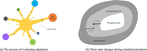
The behavior of slime molds during prey capture can be abstracted into three rules: approaching food, surrounding food, and capturing food (Rizk-Allah et al., 2020). Each iteration process can be divided into three steps: sorting, updating weights, and updating positions. The pseudocode for the SMA is shown in Table 1.
Initialize each parameter: including weights W, maximum number of iterations, etc; Initialize the slime mold population Xi (i = 1, 2, 3 .... , n); For(i=0, Max_Iteration, i++): Determining whether a slime mold individual has exceeded the search space; The starvation value of each slime mold was calculated and ranked to update bestFitness, Xb; Update the weights W by using the following equation:
For each search portion: Update p, vb, vc; Update the position of the slime mold by the following formula:
End for End for Return bestFitness, Xb; |
2.1.3 Algorithmic improvement process
| Serial number | Symbolic | Hidden meaning |
|---|---|---|
| 1 | r | Random number, taking values [0, 1] |
| 2 | W | Weight of the Slime mold |
| 3 | bF | Current iteration optimal fitness value |
| 4 | wF | Worst fitness value of current iteration |
| 5 | Xb(t) | Optimal position of slime mold at tth iteration |
| 6 | ub | Explore space previous session |
| 7 | lb | Explore space next session |
| 8 | vb | Random number taking values [a, −a] |
| 9 | t | Current iteration number |
| 10 | S(i) | Fitness value of the ith individual slime mold |
| 11 | vc | Random number taking values [b, −b] |
| 12 | XA(T), XB(T) | Two randomly selected slime mold individuals in the T iteration |
| 13 | X(t) | Location of the slime mold at the tth iteration |
| 14 | Cω | Nonlinear weights, taking values [0, 1] |
| 15 | Cinitcnp | Initial metacellular neighborhood pheromone |
| 16 | Ccurcnp | Current metacellular neighborhood pheromone |
- Initialization: Create a two-dimensional CA grid where each grid unit represents a cell. Initialize cell states, positions, and algorithm parameters.
- Update weights W, nonlinear weight Cω, and cellular pheromones: Update W, Cω, and cellular pheromones according to Formulas (2) and (6).
- Position update: Use Equation (7) to update the slime mold state to continuously approach the food (endpoint).
- Compute fitness value, and update the global optimal solution based on cellular pheromone concentration.
- Iterate repeatedly to check if termination conditions are met; if not, return to step (2).
- Upon finding food, extract the shortest path information based on the highest cellular pheromone concentration, which represents the shortest path.
2.2 Introduction to comparison algorithms and metrics
2.2.1 Introduction to contrast algorithms
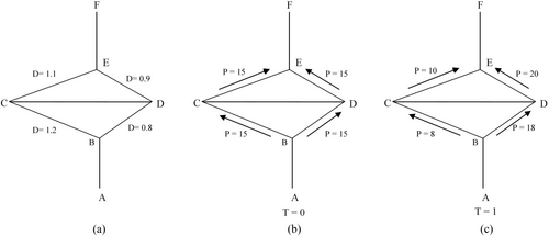
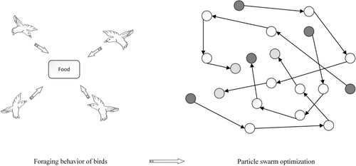
2.2.2 Assessment of indicators
There are three common distance metrics, namely, Euclidean distance (Cheng et al., 2023), Manhattan distance (Tasena, 2022), and Minkowski distance (Zhai et al., 2014). Euclidean distance is the commonly used distance definition, which measures the distance between two points in Euclidean space. It represents the true distance between the two points in an n-dimensional space. Manhattan distance, also known as the city block distance, calculates the sum of the absolute differences between the coordinates of two points in a standard coordinate system. Minkowski distance is not a specific distance itself but rather a general representation of a group of distance metrics. It extends the concepts of Euclidean and Manhattan distances. In this study, the distance metric used in the simulation is Manhattan distance.
3 RESULTS AND ANALYSIS
3.1 Performance test
| No. | ACO | FA | PSO | CASMA | WPA |
|---|---|---|---|---|---|
| 1 | 0.84676876242 | 0.84880630669 | 0.87447750238 | 0.93142489054 | 0.85716971296 |
| 0.86395687683 | 0.89806980602 | 0.95500762799 | 0.94379972422 | 0.8813300155 | |
| 2 | 0.8369587535 | 0.85615864053 | 1.08005364033 | 0.88936464709 | 0.8320238446 |
| 0.77461749315 | 0.75648058412 | 1.12501340197 | 0.7910996943 | 0.77790956349 | |
| 3 | 0.89729124948 | 0.92598109902 | 0.93930852507 | 1.0161456115 | 0.8948083031 |
| 0.90893335673 | 0.9493707060 | 0.9453305244 | 1.16111569333 | 0.92595419910 | |
| 4 | 0.89460482343 | 0.8858373428 | 0.91889646192 | 0.88703115601 | 0.88199031587 |
| 0.84562691568 | 0.89200659686 | 0.8940011153 | 0.89937321436 | 0.88843414192 | |
| 5 | 1.17539253655 | 0.81023276680 | 1.16046827770 | 0.87140644011 | 1.18094921816 |
| 1.29465120566 | 0.78503715564 | 1.33285545883 | 0.79056021797 | 0.73149240970 | |
| 6 | 0.83753634488 | 1.11123468306 | 0.90272264253 | 0.97165820929 | 0.89378208311 |
| 0.89611001387 | 1.15966105279 | 0.87733772010 | 0.96314770539 | 0.87980555494 | |
| 7 | 0.65694620526 | 0.821243674 | 0.69971115407 | 0.78420463012 | 0.70385439276 |
| 0.68312916450 | 0.6512678263 | 0.66110500827 | 0.79659943133 | 0.71431500129 | |
| 8 | 0.94943194466 | 0.96057169014 | 0.9629665491 | 0.98764099224 | 0.96645008869 |
| 0.89777682379 | 0.96891076039 | 0.97799054029 | 0.96986277490 | 0.91551616124 | |
| 9 | 0.88188950731 | 0.88059598142 | 0.8437905036 | 1.03997546824 | 0.88263647376 |
| 0.80720280508 | 0.75897106029 | 0.90676500247 | 1.29388133884 | 0.77633867026 | |
| 10 | 1.35940645753 | 1.06866189224 | 1.06364366798 | 1.09870001903 | 1.07633846745 |
| 1.39581394123 | 1.117416925336 | 1.14508501980 | 1.29602459490 | 1.29846148467 |
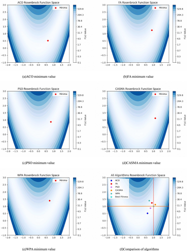
As shown in Figure 5, panels (a), (b), (c), (d), and (e) represent the minimum value results obtained after 500 iterations of the ACO, FA, PSO, CASMA, and WPA algorithms, respectively, on the Rosenbrock test function. Figure 5f illustrates the distribution of the minimum values obtained by the five algorithms. The optimal value for the objective function is (1, 1). From the graph, it can be observed that after 500 iterations, the solution obtained by CASMA is closest to (1, 1), indicating that CASMA outperforms the other four algorithms in terms of value accuracy.
From Table 3, it can be seen that CASMA has smaller fluctuations compared with the other four algorithms in the 10 value results and the overall results are closer to the optimal value.
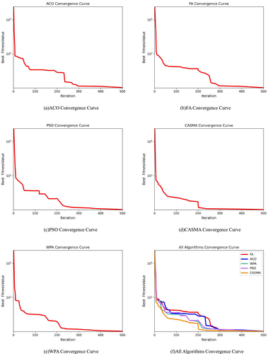
As depicted in Figure 6, panels (a), (b), (c), (d), and (e) represent the convergence curves of ACO, FA, PSO, CASMA, and WPA, respectively, during the iterative process on the Rosenbrock test function. Panel (f) provides a comparative analysis of the convergence curves for the five algorithms. From the graph, it is evident that CASMA exhibits a rapid descent in the convergence curve before approximately 50 iterations, reaching convergence around the 200th iteration. The convergence speed of CASMA is observed to be faster than the other four algorithms, and it achieves higher precision in the obtained values.
3.2 Simulation and result analysis
In order to simulate the obstacle avoidance and path planning performance of the manure-cleaning robot in a realistic environment, three maps with varying complexities were designed for simulation experiments. The simulations were implemented using Python3 on a Windows laptop equipped with an Intel Core i5-12450H and NVIDIA GeForce 3060 Laptop, and the simulation setup details can be found in Table 4. To ensure fairness, parameters such as start and end points, iteration count, and initial population size were consistent across each map. The specific simulated pig farm environments are outlined as follows: Map 1, depicted in Figure 7, simulates the path planning performance of the manure-cleaning robot in a pigpen with three randomly distributed pigs; Map 2, illustrated in Figure 8, simulates the scenario with seven randomly distributed pigs; and Map 3, shown in Figure 9, simulates the situation with 12 randomly distributed pigs. Each algorithm was run 500 times in each environment (three maps) to obtain simulation results, demonstrating the repeatability of the CASMA method. Table 5 presents the percentage of steps saved by CASMA compared with the four contrasting algorithms, whereas Table 6 provides the percentage of processing time saved by CASMA compared with the four contrasting algorithms.
| Basic hardware information | Version |
|---|---|
| Processor | Intel Core i5-12450H |
| Graphics card | NVIDIA GeForce 3060 Laptop |
| Memory | 16G |
| Hard disk | 512G SSD |
| Basic software information | Version |
|---|---|
| Anaconda | Anaconda3 2019.10(64-bit) |
| Python | 3.7 |
| Numpy | 1.21.6 |
| Matplotlib | 3.5.3 |
| Operating system | Windows11 |
| Map number | CASMA-ACO | CASMA-FA | CASMA-PSO | CASMA-WPA |
|---|---|---|---|---|
| Percentage reduction in step consumption (%) | Percentage reduction in step consumption (%) | Percentage reduction in step consumption (%) | Percentage reduction in step consumption (%) | |
| 1 | 5.97 | 1.56 | 0.0 | 3.07 |
| 2 | 8.45 | 1.51 | 2.98 | 9.72 |
| 3 | 9.67 | 1.75 | 0.0 | 0.0 |
| Map number | CASMA-ACO | CASMA-FA | CASMA-PSO | CASMA-WPA |
|---|---|---|---|---|
| Percentage savings in processing time (%) | Percentage savings in processing time (%) | Percentage savings in processing time (%) | Percentage savings in processing time (%) | |
| 1 | 16.28 | 23.01 | 9.15 | 4.94 |
| 2 | 9.30 | 13.10 | 4.00 | 5.60 |
| 3 | 14.03 | 24.22 | 19.45 | 8.66 |
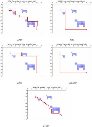
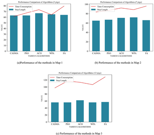
In Map 1, where three pigs are randomly distributed, the performance of the manure-cleaning robot in a map of simple complexity was simulated using five metaheuristic algorithms. All algorithms utilized the same starting point for the robot (coordinates x, y = 9, 9, indicated by a blue dot) and the destination point for waste cleaning (coordinates x, y = 40, 40, indicated by a green dot). CASMA ultimately found an optimal path with a step count of 63, taking a total of 61.227 ms. In comparison with ACO, FA, and WPA, CASMA demonstrated step savings of 5.97%, 1.56%, and 3.07%, respectively, and time savings of 16.28%, 23.01%, and 4.94%, respectively. Compared with PSO, although the step count remained the same, CASMA achieved a time saving of 9.15%.
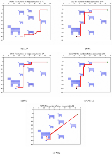
In Map 2, simulating a map of higher complexity with seven randomly distributed pigs, the path planning performance of five metaheuristic algorithms was evaluated. The robot's initial position in the map was set at x, y = 12, 40, and the waste cleaning point was located at x, y = 42, 6. CASMA ultimately devised a path with a step count of 65, taking 83.441 ms. In comparison with ACO, FA, PSO, and WPA, CASMA demonstrated step savings of 8.45%, 1.51%, 2.98%, and 9.72%, respectively. Time savings were observed at 9.30%, 13.10%, 4.00%, and 5.60%.
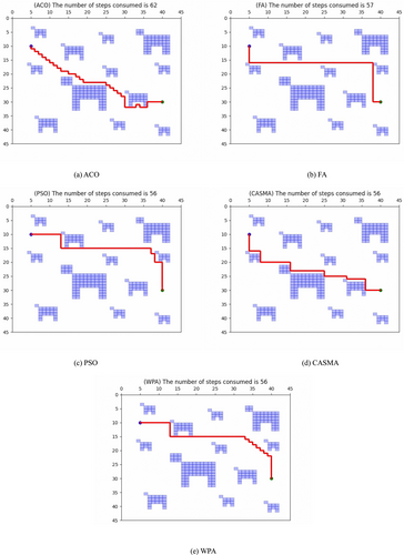
In Map 3, where 12 pigs are randomly distributed, the performance of the manure-cleaning robot in a complex environment was simulated using five metaheuristic algorithms. The robot's initial position in the map was set at x, y = 5, 10, and the waste cleaning point was located at x, y = 40, 30. CASMA ultimately devised a path with a step count of 56, taking 83.441 ms. Compared with ACO and FA, CASMA demonstrated step savings of 9.67% and 1.75%, respectively. Time savings were observed at 14.03% and 24.22%, respectively. Although the step count remained the same as PSO and WPA, CASMA maintained an advantage in time consumption, with time savings of 19.45% and 8.66%, respectively.
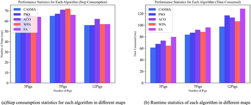
In summary, the simulation results demonstrate that CASMA holds an advantage over the other four metaheuristic algorithms in both step count and processing time during the path planning process. Detailed data obtained from the aforementioned simulations are presented in Table 7. Figure 10a,b,c depicts the step count and time consumption of each algorithm under the three different maps, whereas Figure 11a,b provides a consolidated comparison of step count and time consumption. Some parameters set during the simulation of the five metaheuristic algorithms are listed in Table 8.
| Arithmetic | Number of pigs | Position of each pig (X, Y-coordinate, size of pig) | Coordinates of the robot's location | Coordinates of feces | Number of steps consumed | Processing time (ms) | Path (X-axis coordinates) | Path (Y-axis coordinates) |
|---|---|---|---|---|---|---|---|---|
| CASMA | 3 |
[33,31,9] [13,14,3] [25,11,5] |
(9,9) |
(40,40) |
63 | 61.2278 | [9, 9, 9, 9, 9, 9, 9, 9, 9, 9, 9, 9, 9, 9, 9, 9, 9, 9, 9, 9, 9, 9, 9, 9, 9, 9, 9, 9, 9, 9, 9, 9, 10, 11, 12, 13, 14, 15, 16, 17, 18, 19, 20, 21, 22, 23, 24, 25, 26, 27, 28, 29, 30, 31, 32, 33, 34, 35, 36, 37, 38, 39, 40] | [9, 10, 11, 12, 13, 14, 15, 16, 17, 18, 19, 20, 21, 22, 23, 24, 25, 26, 27, 28, 29, 30, 31, 32, 33, 34, 35, 36, 37, 38, 39, 40, 40, 40, 40, 40, 40, 40, 40, 40, 40, 40, 40, 40, 40, 40, 40, 40, 40, 40, 40, 40, 40, 40, 40, 40, 40, 40, 40, 40, 40, 40, 40] |
| PSO | 63 | 67.3993 | [9, 10, 11, 12, 13, 14, 15, 16, 17, 18, 19, 20, 21, 22, 22, 22, 22, 22, 22, 23, 24, 25, 26, 27, 28, 29, 30, 31, 32, 33, 34, 35, 36, 37, 38, 39, 40, 40, 40, 40, 40, 40, 40, 40, 40, 40, 40, 40, 40, 40, 40, 40, 40, 40, 40, 40, 40, 40, 40, 40, 40, 40, 40] | [9, 9, 9, 9, 9, 9, 9, 9, 9, 9, 9, 9, 9, 9, 10, 11, 12, 13, 14, 14, 14, 14, 14, 14, 14, 14, 14, 14, 14, 14, 14, 14, 14, 14, 14, 14, 14, 15, 16, 17, 18, 19, 20, 21, 22, 23, 24, 25, 26, 27, 28, 29, 30, 31, 32, 33, 34, 35, 36, 37, 38, 39, 40] | ||||
| FA | 64 | 79.5265 | [9, 10, 11, 12, 13, 14, 15, 15, 15, 15, 15, 15, 15, 15, 15, 15, 15, 15, 15, 15, 15, 15, 15, 15, 15, 15, 15, 15, 15, 15, 15, 15, 15, 15, 15, 15, 15, 15, 16, 17, 18, 19, 20, 21, 22, 23, 24, 25, 26, 27, 28, 29, 30, 31, 32, 33, 34, 35, 36, 37, 38, 39, 40, 40] | [9, 9, 9, 9, 9, 9, 9, 10, 11, 12, 13, 14, 15, 16, 17, 18, 19, 20, 21, 22, 23, 24, 25, 26, 27, 28, 29, 30, 31, 32, 33, 34, 35, 36, 37, 38, 39, 40, 40, 40, 40, 40, 40, 40, 40, 40, 40, 40, 40, 40, 40, 40, 40, 40, 40, 40, 40, 40, 40, 40, 40, 40, 40, 40] | ||||
| WPA | 65 | 64.4125 | [9, 9, 9, 10, 10, 11, 11, 12, 12, 13, 14, 15, 15, 15, 15, 16, 16, 17, 17, 18, 18, 19, 19, 20, 20, 21, 21, 22, 22, 23, 23, 24, 24, 25, 25, 25, 25, 25, 26, 26, 27, 28, 28, 28, 28, 28, 28, 28, 28, 29, 30, 31, 32, 33, 34, 35, 36, 37, 37, 38, 38, 39, 39, 40, 40, 40] | [9, 10, 11, 11, 12, 12, 11, 11, 12, 12, 12, 12, 13, 14, 15, 15, 16, 16, 17, 17, 18, 18, 19, 19, 20, 20, 21, 21, 22, 22, 23, 23, 24, 24, 25, 26, 27, 28, 28, 29, 29, 29, 30, 31, 32, 33, 34, 35, 36, 36, 36, 36, 36, 36, 36, 36, 36, 36, 37, 37, 38, 38, 39, 39, 40, 41] | ||||
| ACO | 67 | 73.1416 | [9, 8, 8, 9, 10, 11, 11, 12, 13, 14, 15, 15, 15, 15, 15, 15, 15, 16, 17, 18, 19, 20, 20, 20, 20, 21, 22, 23, 24, 25, 26, 27, 28, 29, 29, 29, 29, 29, 29, 29, 29, 30, 31, 32, 33, 34, 35, 36, 37, 38, 39, 40, 41, 41, 41, 41, 41, 41, 41, 41, 40, 40, 40, 40, 40, 40, 40] | [9, 9, 10, 10, 10, 10, 11, 11, 11, 11, 11, 12, 13, 14, 15, 16, 17, 17, 17, 17, 17, 17, 18, 19, 20, 20, 20, 20, 20, 20, 20, 20, 20, 20, 21, 22, 23, 24, 25, 26, 27, 27, 27, 27, 27, 27, 27, 27, 27, 27, 27, 27, 27, 28, 29, 30, 31, 32, 33, 34, 34, 35, 36, 37, 38, 39, 40] | ||||
| CASMA | 7 |
[11,33,9] [26,16,5] [17,9,5] [17, 22,3] [25,7,3] [38,21,5] [26,35,5] |
(12,40) |
(42,6) |
65 | 83.4416 | [12, 12, 12, 13, 14, 15, 16, 16, 16, 16, 16, 16, 16, 16, 16, 16, 16, 16, 16, 16, 16, 17, 18, 19, 19, 19, 19, 19, 19, 19, 19, 19, 19, 19, 19, 19, 20, 20, 20, 20, 21, 22, 23, 24, 25, 26, 27, 27, 27, 27, 28, 29, 30, 31, 32, 33, 34, 35, 36, 37, 38, 39, 40, 41, 42] | [40, 39, 38, 38, 38, 38, 38, 37, 36, 35, 34, 33, 32, 31, 30, 29, 28, 27, 26, 25, 24, 24, 24, 24, 23, 22, 21, 20, 19, 18, 17, 16, 15, 14, 13, 12, 12, 11, 10, 9, 9, 9, 9, 9, 9, 9, 9, 8, 7, 6, 6, 6, 6, 6, 6, 6, 6, 6, 6, 6, 6, 6, 6, 6, 6] |
| PSO | 67 | 86.9187 | [12, 12, 12, 13, 14, 14, 15, 16, 17, 18, 19, 19, 19, 19, 19, 19, 19, 19, 19, 19, 19, 19, 19, 19, 19, 19, 19, 19, 19, 19, 19, 19, 19, 19, 19, 19, 19, 19, 20, 20, 20, 20, 21, 22, 23, 24, 25, 26, 27, 27, 27, 27, 28, 29, 30, 31, 32, 33, 34, 35, 36, 37, 38, 39, 40, 41, 42] | [40, 39, 38, 38, 38, 39, 39, 39, 39, 39, 39, 38, 37, 36, 35, 34, 33, 32, 31, 30, 29, 28, 27, 26, 25, 24, 23, 22, 21, 20, 19, 18, 17, 16, 15, 14, 13, 12, 12, 11, 10, 9, 9, 9, 9, 9, 9, 9, 9, 8, 7, 6, 6, 6, 6, 6, 6, 6, 6, 6, 6, 6, 6, 6, 6, 6,6] | ||||
| FA | 66 | 96.0231 | [12, 13, 14, 15, 16, 16, 16, 16, 16, 16, 16, 16, 16, 16, 16, 16, 16, 16, 16, 16, 16, 17, 18, 19, 20, 20, 20, 20, 20, 20, 20, 20, 20, 20, 20, 20, 20, 20, 20, 20, 21, 22, 23, 24, 25, 26, 27, 27, 27, 27, 28, 29, 30, 31, 32, 33, 34, 35, 36, 37, 38, 39, 40, 41, 42, 42] | [40, 40, 40, 40, 40, 39, 38, 37, 36, 35, 34, 33, 32, 31, 30, 29, 28, 27, 26, 25, 24, 24, 24, 24, 24, 23, 22, 21, 20, 19, 18, 17, 16, 15, 14, 13, 12, 11, 10, 9, 9, 9, 9, 9, 9, 9, 9, 8, 7, 6, 6, 6, 6, 6, 6, 6, 6, 6, 6, 6, 6, 6, 6, 6, 6, 6] | ||||
| WPA | 72 | 88.3926 | [12, 12, 12, 12, 12, 12, 13, 13, 13, 13, 13, 14, 15, 16, 16, 16, 16, 16, 16, 16, 16, 17, 17, 18, 18, 19, 19, 20, 20, 21, 21, 22, 22, 23, 23, 24, 24, 25, 25, 26, 26, 27, 27, 28, 28, 29, 29, 30, 30, 31, 31, 32, 32, 33, 33, 34, 34, 35, 35, 36, 36, 37, 37, 38, 38, 39, 39, 40, 40, 41, 41, 42, 42] | [40, 39, 38, 37, 36, 35, 35, 36, 37, 38, 39, 39, 39, 39, 38, 37, 36, 35, 34, 33, 32, 32, 31, 31, 30, 30, 29, 29, 28, 28, 27, 27, 26, 26, 25, 25, 24, 24, 23, 23, 22, 22, 21, 21, 20, 20, 19, 19, 18, 18, 17, 17, 16, 16, 15, 15, 14, 14, 13, 13, 12, 12, 11, 11, 10, 10, 9, 9, 8, 8, 7, 7, 6] | ||||
| ACO | 71 | 92.0016 | [12, 12, 13, 14, 15, 16, 16, 17, 18, 18, 19, 20, 20, 20, 20, 21, 22, 23, 24, 25, 26, 27, 28, 29, 29, 30, 31, 31, 32, 32, 32, 33, 34, 35, 36, 36, 36, 36, 36, 36, 36, 36, 36, 36, 36, 36, 36, 36, 36, 35, 35, 35, 35, 35, 35, 35, 35, 35, 35, 35, 35, 35, 35, 35, 36, 37, 38, 39, 40, 41, 42] | [40, 41, 41, 41, 41, 41, 40, 40, 40, 41, 41, 41, 40, 39, 38, 38, 38, 38, 38, 38, 38, 38, 38, 38, 37, 37, 37, 36, 36, 35, 34, 34, 34, 34, 34, 33, 32, 31, 30, 29, 28, 27, 26, 25, 24, 23, 22, 21, 20, 20, 19, 18, 17, 16, 15, 14, 13, 12, 11, 10, 9, 8, 7, 6, 6, 6, 6, 6, 6, 6, 6] | ||||
| CASMA | 12 |
[20,28,9] [7,5,5] [16,12,3] [6,18,3] [25,7,3] [26,19,3] [40,18,3] [39, 9,7] [33,29,5] [9,38,5] [28,38,3] [40,40,3] |
(5,10) |
(40,30) |
56 | 97.4216 | [5, 5, 5, 5, 5, 5, 5, 6, 7, 8, 8, 8, 8, 8, 9, 10, 11, 12, 13, 14, 15, 16, 16, 16, 16, 17, 18, 19, 20, 21, 22, 23, 24, 25, 25, 25, 26, 27, 28, 29, 30, 31, 31, 32, 33, 34, 35, 36, 36, 36, 36, 36, 37, 38, 39, 40] | [10, 11, 12, 13, 14, 15, 16, 16, 16, 16, 17, 18, 19, 20, 20, 20, 20, 20, 20, 20, 20, 20, 21, 22, 23, 23, 23, 23, 23, 23, 23, 23, 23, 23, 24, 25, 25, 25, 25, 25, 25, 25, 26, 26, 26, 26, 26, 26, 27, 28, 29, 30, 30, 30, 30, 30] |
| PSO | 56 | 116.8793 | [5, 6, 7, 8, 9, 10, 11, 12, 13, 13, 13, 13, 13, 13, 14, 15, 16, 17, 18, 19, 20, 21, 22, 23, 24, 25, 26, 27, 28, 29, 30, 31, 32, 33, 34, 35, 36, 37, 37, 37, 38, 38, 38, 38, 39, 40, 40, 40, 40, 40, 40, 40, 40, 40, 40,40] | [10, 10, 10, 10, 10, 10, 10, 10, 10, 11, 12, 13, 14, 15, 15, 15, 15, 15, 15, 15, 15, 15, 15, 15, 15, 15, 15, 15, 15, 15, 15, 15, 15, 15, 15, 15, 15, 15, 16, 17, 17, 18, 19, 20, 20, 20, 21, 22, 23, 24, 25, 26, 27, 28, 29,30] | ||||
| FA | 57 | 128.5698 | [5, 5, 5, 5, 5, 5, 5, 6, 7, 8, 9, 10, 11, 12, 13, 14, 15, 16, 17, 18, 19, 20, 21, 22, 23, 24, 25, 26, 27, 28, 29, 30, 31, 32, 33, 34, 35, 36, 37, 38, 38, 38, 38, 38, 38, 38, 38, 38, 38, 38, 38, 38, 38, 38, 39, 40, 40] | [10, 11, 12, 13, 14, 15, 16, 16, 16, 16, 16, 16, 16, 16, 16, 16, 16, 16, 16, 16, 16, 16, 16, 16, 16, 16, 16, 16, 16, 16, 16, 16, 16, 16, 16, 16, 16, 16, 16, 16, 17, 18, 19, 20, 21, 22, 23, 24, 25, 26, 27, 28, 29, 30, 30, 30, 30] | ||||
| WPA | 57 | 106.6587 | [5, 6, 7, 8, 9, 10, 11, 12, 13, 13, 13, 13, 13, 13, 14, 15, 16, 17, 18, 19, 20, 21, 22, 23, 24, 25, 26, 27, 28, 29, 30, 31, 32, 33, 33, 34, 34, 35, 35, 36, 36, 37, 37, 38, 38, 39, 39, 40, 40, 40, 40, 40, 40, 40, 40, 40] | [10, 10, 10, 10, 10, 10, 10, 10, 10, 11, 12, 13, 14, 15, 15, 15, 15, 15, 15, 15, 15, 15, 15, 15, 15, 15, 15, 15, 15, 15, 15, 15, 15, 15, 16, 16, 17, 17, 18, 18, 19, 19, 20, 20, 21, 21, 22, 22, 23, 24, 25, 26, 27, 28, 29, 30] | ||||
| ACO | 62 |
113.3314 |
[5, 5, 6, 6, 7, 7, 8, 8, 9, 9, 10, 10, 11, 11, 12, 12, 13, 13, 14, 15, 15, 16, 17, 17, 18, 18, 19, 19, 20, 21, 22, 23, 24, 25, 25, 26, 26, 27, 27, 28, 28, 29, 29, 30, 30, 30, 30, 30, 31, 32, 33, 33, 34, 34, 35, 36, 36, 36, 37, 38, 39, 40] | [10, 11, 11, 12, 12, 13, 13, 14, 14, 15, 15, 16, 16, 17, 17, 18, 18, 19, 19, 19, 20, 20, 20, 21, 21, 22, 22, 23, 23, 23, 23, 23, 23, 23, 24, 24, 25, 25, 26, 26, 27, 27, 28, 28, 29, 30, 31, 32, 32, 32, 32, 31, 31, 32, 32, 32, 31, 30, 30, 30, 30, 30] |
| No. | Parameter name | Specific parameter value | ||||
|---|---|---|---|---|---|---|
| WPA | ACO | PSO | FA | CASMA | ||
| 1 | Number of iterations | 500 | 500 | 500 | 500 | 500 |
| 2 | Wolf pack size | 100 | - | - | - | - |
| 3 | Contraction factor (walpha) | 0.5 | - | - | - | - |
| 4 | Explore the parameters (wbeta) | 0.3 | - | - | - | - |
| 5 | Number of Ants | - | 100 | - | - | - |
| 6 | Pheromone concentration | - | 1 | - | - | - |
| 7 | Pheromone evaporation rate | - | 0.5 | - | - | - |
| 8 | Number of particles | - | - | 100 | - | - |
| 9 | Inertia weight | - | - | 5 | - | - |
| 10 | Cognitive rate | - | - | 1.5 | - | - |
| 11 | Social rate | - | 1.6 | - | - | |
| 12 | Number of fireflies | - | - | - | 100 | - |
| 13 | Light intensity decay factor (gamma) | - | - | - | 1 | - |
| 14 | Attraction factor (falpha) | - | - | - | 0.2 | - |
| 15 | Number of slime mold populations | - | - | - | - | 100 |
| 16 | The proportion of individuals with random number distribution to the total (Z) | - | - | - | - | 0.3 |
| 17 | Dimensions | - | - | - | - | 2 |
In practical pig farming scenarios, pigs move randomly, necessitating continual adjustment and replanning of the remaining path for the cleaning robot as it navigates the environment. This dynamic process involves responding to changes in pig positions on the map. To evaluate CASMA's performance in real-world settings, a dynamic obstacle experiment was designed and compared against commonly used heuristic algorithms for path planning, namely, A* and TS. TS incorporates neighborhood interaction concepts similar to CA's best neighborhood movement rules and tabu list updates. In the dynamic obstacle experiment, each pig's position within the map changes randomly over time (with random direction and distance of movement). Consequently, the cleaning robot must replan its optimal path with each step it takes, continuing until it reaches the cleaning point (where reaching the point marks one trial). After reaching the cleaning point, the path length covered and the total time consumed for multiple path planning instances are measured for performance comparison. Simulation experiments were conducted on the three maps described in Table 7, each simulating 12 pigs randomly distributed as in Figure 9. The experimental setup and CASMA parameters remained consistent with the previous sections, conducting 500 repeated trials on each map (a total of 1500 trials across the three maps) to ensure the reliability of the results. Figure 12 illustrates the pathfinding process of the robot during the dynamic obstacle experiment. Table 9 presents selected experimental data and the average path planning time and step consumption of CASMA after 1500 trials across the three maps. Figure 13 provides a statistical summary of the results from 500 repeated trials of the three algorithms on map one.

| CASMA | A* | TS | ||||
|---|---|---|---|---|---|---|
| Total time consumed for route planning (ms) | Total steps consumed (step) | Total time consumed for route planning (ms) | Total steps consumed (step) | Total time consumed for route planning (ms) | Total steps consumed (step) | |
Map 1 Robot location (9,9); Fecal location (40,40) |
18 262.65 | 256 | 39 947.33 | 289 | 42 379.12 | 277 |
| 17 359.60 | 238 | 37 918.58 | 271 | 44 308.00 | 288 | |
| 20 015.72 | 269 | 34 959.95 | 260 | 36 910.66 | 239 | |
Map 2 Robot location (12,40); Fecal location (42,6) |
19 550.50 | 269 | 36 520.82 | 268 | 43 786.29 | 281 |
| 21 551.94 | 285 | 39 101.74 | 287 | 40 233.78 | 255 | |
| 19 978.07 | 276 | 41 449.76 | 301 | 39 663.90 | 250 | |
Map 3 Robot position (5, 10); Fecal position (40, 30) |
12 385.94 | 165 | 21 150.85 | 173 | 29 516.10 | 171 |
| 15 569.01 | 186 | 29 980.76 | 208 | 33 792.86 | 203 | |
| 10 816.42 | 137 | 19 058.04 | 171 | 30 668.22 | 178 | |
| Average consumption over 1500 iterations | 16 919.29 | 237.70 | 32 710.59 | 241.92 | 38 706.78 | 239.66 |

The experimental results above demonstrate that after 1500 repeated trials, CASMA exhibited an average total time consumption of 16,919.29 ms. Compared with A* and TS, CASMA achieved average time savings of 48.27% and 56.28%, respectively. Regarding total step consumption, CASMA also saved 1.74% and 0.81% compared with A* and TS. These findings indicate that CASMA significantly reduces algorithm response time while ensuring sufficiently short movement paths for the robot. This makes CASMA well-suited for applications in pig farming environments characterized by complexity, variable obstacles, and the need for prompt responses to pig movements.
4 DISCUSSION
4.1 Real-world applicability
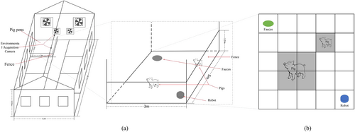
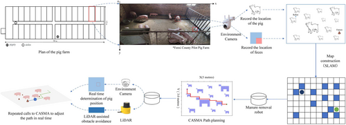
- Every 3 h, the system initiates a manure-cleaning operation: Cameras positioned above the pigsty automatically record the locations of pig waste and pigs. The position data are then transmitted to the robot, utilizing Xiaomi CW500 devices (model MJSXJ07HL).
- Based on positional information, the robot utilizes its onboard cameras and laser rangefinder sensor (model DST700) in conjunction with environmental cameras to collect data, employing the SLAM algorithm for mapping and map building.
- Environmental cameras continuously monitor changes in pig positions, facilitating real-time data exchange between the robot's own sensors and its operations, thereby updating pig locations on the map in real time.
- Leveraging the current location, positions of pig waste, and pig locations, the robot utilizes CASMA (Cellular Automaton-based Spatial Multi-Agent system) for path planning.
- Following the planned path and assisted by laser rangefinders for obstacle detection, the robot iteratively executes steps (3) and (4), adjusting the optimal route to ultimately reach the designated cleaning points.
| 8:00 a.m. | 11:00 a.m. | 14:00 p.m. | 17:00 p.m. | 20:00 p.m. | ||||||
|---|---|---|---|---|---|---|---|---|---|---|
| Start(2,11)End(19,2) | Start(1,1)End(10,5) | Start(4,5)End(20,12) | Start(3,10)End(18,1) | Start(5,5)End(10,9) | ||||||
| Simulated experiment | Actual consumption | Simulated experiment | Actual consumption | Simulated experiment | Actual consumption | Simulated experiment | Actual consumption | Simulated experiment | Actual consumption | |
| Processing time (ms) | 106.31 | 111.58 | 76.62 | 81.24 | 95.55 | 105.18 | 99.91 | 110.56 | 61.13 | 69.46 |
| Number of steps consumed | 26 | 31 | 13 | 14 | 23 | 27 | 24 | 27 | 9 | 13 |
- Note: The results in the table are the first path information planned by the robot after it starts working based on the location of the manure and the location of the pigs in the barn recorded by the environmental camera.
The above test results demonstrate a close correlation between the actual path planning performance of the robot equipped with CASMA and the algorithm's simulated experimental outcomes. This confirms the feasibility and effectiveness of applying CASMA to achieve efficient waste removal operations through shortest path planning for pig excrement-cleaning robots.
4.2 Analysis of economic benefits
Traditional pigsty manure cleaning relies on manual labor, demanding a significant workforce, a challenge exacerbated by urbanization in many countries leading to a sharp decline in agricultural labor. Aging rural labor further compounds this issue. In developed nations, high labor costs render employing large human resources for manure cleaning impractical. For a large pig farm measuring 60–80 m long and 20–30 m wide, employing two to three workers daily for cleaning at $30 USD per person per day totals monthly labor costs of $1800–2700 USD. With the potential application of this research, labor costs become negligible. Regarding equipment expenses, a laser obstacle avoidance radar costs about $280 USD, a camera approximately $40 USD, and networking equipment and workstations totaling about $2485 USD, plus miscellaneous consumables, summing up to around $3452 USD, roughly equivalent to 45 days of labor costs. Overall, although initial investment in adopting a manure-cleaning robot may be higher compared with labor costs, long-term operational expenses are significantly lower.
Furthermore, research indicates significant economic benefits, with a profit of 48.5 RMB per ton of managed pig manure (Shi et al., 2023). For instance, in a medium-sized pig farm with 1000 pigs, each finishing pig produces 2–3 kg of manure daily, resulting in 2–3 tons of manure per day. This translates to daily profits from manure management amounting to 98–145.5 RMB, approximately $13–20 USD. Therefore, this study underscores substantial economic implications.
4.3 Analysis of model limitations
CASMA demonstrates rapid capability in identifying optimal paths to manure-cleaning points within complex real-world pig farm environments. However, applying it to achieve precise feces cleaning with pig farm robots presents a formidable challenge. This challenge primarily arises from CASMA's dependence on the accuracy of the environmental model; deviations or incompleteness in the model can significantly impact algorithm performance. In this study, pigs' presence on the map is represented as obstacle grid cells, without accurately extracting the contours of the pigs themselves. The routes planned by CASMA are contingent upon the partitioning of the map into grid cells of varying sizes and quantities, necessitating further experimental validation of their practical implications. Moreover, despite substantial improvements in convergence speed and search accuracy, the algorithm may still encounter a balance issue between local and global search in environments of unexpected complexity. Additionally, as a metaheuristic algorithm, CASMA involves initial parameter settings, and different parameter configurations can affect the model's actual performance. Optimal parameter selection requires extensive experimental verification. Lastly, there are concerns regarding the algorithm's general applicability. CASMA is designed specifically for the path planning of pig farm cleaning robots, and its suitability for other domains or different problems remains to be further validated.
5 CONCLUSIONS
The presented work introduces an improved slime mold algorithm CASMA, applied to path planning for a robotic swine manure-cleaning system. This algorithm efficiently generates a collision-free optimal path to reach manure-cleaning points in a relatively short time. Three pig group densities, ranging from low to high, are set to simulate the distribution of pigs in real scenarios, using Python for simulation. The simulation results demonstrate that CASMA reduces average step consumption by 8.03%, 1.61%, 0.99%, and 4.26% compared with four metaheuristic algorithms (ACO, FA, PSO, and WPA, respectively) and average processing time by 13.20%, 20.11%, 10.86%, and 6.4%, respectively. Experimental validation with dynamic obstacles confirms that CASMA effectively navigates around moving pigs during actual waste-cleaning tasks, reaching cleaning sites with minimal steps. Furthermore, compared with A* and TS heuristic algorithms, CASMA achieves an average reduction of 48.27% and 56.28% in total path planning time, significantly enhancing the response speed of waste-cleaning robots. In summary, CASMA not only optimizes the optimal path to waste cleaning points but also outperforms other algorithms in terms of minimal cost and computational requirements, establishing a foundation for collision-free path planning of waste cleaning robots in pig farms. This approach effectively reduces or prevents collisions between robots and pigs, maintaining clean pig pens, improving the living environment and welfare of pigs, and enhancing productivity in the meat production industry. Additionally, this study demonstrates the effectiveness of using cellular automata as an enhancement method, combined with metaheuristic algorithms to improve algorithm convergence speed and precision. Future research will further validate CASMA's performance in practical waste cleaning operations, investigate the effects of cell size in map partitioning and different algorithm parameter settings on performance, and explore multimodal fusion methods such as image and infrared integration for environmental recognition, obstacle avoidance, and map establishment in highly complex pigsty environments. Integration of CASMA aims to facilitate rapid and accurate waste cleaning operations by robotic systems in such challenging environments.
CONFLICT OF INTEREST STATEMENT
The authors declare no conflicts of interest for this article.


