Reaction-norm animal model analysis of average daily gain heat tolerance in purebred Duroc pigs
Abstract
The present study aimed to genetically improve growth performance under high-heat environments by specifically designing a reaction-norm animal model (RNAM) for purebred Duroc pigs in Japan. A total of 54,750 records of average daily gain (ADG) measured for pigs reared at four farms in different prefectures were analyzed. Estimated maximum daily temperatures at the respective farm locations were used to calculate the average cumulative thermal load (TL). The TL values served as an indicator of high-heat environments for pigs. The plausible cumulative period length and threshold temperature for calculating TL were determined to be 8 weeks until just before shipping and 25°C, respectively. Variance components were estimated via RNAM analysis using TL as a linear covariate. The estimated additive genetic variances under both responsive and non-responsive to TL were found to be significant. Moreover, the estimated heritability of ADG ranged from 0.38 to 0.73 for TL values of 0–8. These results suggest that the RNAM developed holds the potential for improving the genetic ability of growth under high-heat environments in pigs.
1 INTRODUCTION
Global warming has a tremendous negative impact on the overall sustainability of pig production (Mayorga et al., 2019; Ramirez et al., 2022). In Japan, Takada et al. (2008) predicted a decrease in the future growth performance of pigs in most areas because of ongoing global warming. To mitigate the impact of elevated ambient temperatures, various countermeasures have been implemented, including improving the rearing environment in piggery facilities and adjusting the nutrient composition of feeds (Liu et al., 2022; Mayorga et al., 2019). However, as global warming becomes more severe, the cost of pork production may increase owing to reduced productivity (Mayorga et al., 2019). Therefore, ensuring stable pork production under high-heat weather conditions is important.
To identify high-heat environment indicators in pigs, obtaining accurate and actual environmental information is desirable. However, comprehensive on-farm environmental data have not been continuously collected on many farms in Japan. Notably, meteorological observatory data have been accumulated at weather stations located across Japan. In other countries, various studies have been conducted on genetically improving heat tolerance using growth performance and publicly available weather records in pig populations (Fragomeni et al., 2016; Freitas et al., 2023; Usala et al., 2021; Zumbach et al., 2008a). Recently, in Japan, the availability of public weather records and their association with pig production records have been also assessed (Hara et al., 2022; Ogawa et al., 2022; Sasaki et al., 2018; Satoh et al., 2023, 2023).
Genetic improvement of heat tolerance in pigs could serve as an effective strategy for addressing the challenges posed by global warming (Mayorga et al., 2019). To achieve this, a statistical model that considers the genotype by environment interaction (G × E) is essential to evaluate the genetic transmitting ability of heat tolerance. One such model is the reaction-norm model (RNM), a type of random regression framework. The RNM can distinguish between genetic effects that respond to environmental indicators and genetic effect that do not (Cardoso & Tempelman, 2012; Mulder et al., 2006; Via et al., 1995). The Duroc is a popular terminal sire breed around the world. Previous studies have performed reaction-norm sire model analyses on crossbred pig populations with Duroc as the sire breed (Fragomeni et al., 2016; Usala et al., 2021; Zumbach et al., 2008a), as well as reaction-norm animal model (RNAM) analysis using records obtained from purebred Duroc pigs (Fragomeni et al., 2016).
In this study, we aimed to investigate the potential for genetically improving growth performance under high-heat environments using the purebred Duroc pig records in Japan. Initially, we employed regression analysis to construct a model in which average daily gain (ADG) decreased with high-heat environment indicators. Subsequently, we conducted RNAM analysis considering high-heat environment indicators to estimate genetic parameters and predict breeding values. Finally, we discussed the possibility of improving growth performance under high-heat environmental conditions.
2 MATERIALS AND METHODS
2.1 Records
Pedigree and growth performance records were collected from the four-member producer farms (Figure S1) of Global Pig Farms Incorporated (Shibukawa, Japan). The farms are located at latitudes 35.3–43.0°N and longitudes 137.4–141.6°E and are scattered from central to northern Japan. It is important to note that one of the four farms (Farm D) was not included in several results because the growth performance records were not collected after 2020. The trait studied was the average daily gain (ADG, g/day), calculated by dividing the body weight (BW, kg) by the age in days at the end of performance testing. Typically, the performance testing concludes when BW reaches 105 kg. Moreover, ADG records deviating by three standard deviations from the mean were excluded. Contemporary groups were defined by birth farm × year × bi-monthly season (). Subsequently, records of contemporary groups where fewer than 10 pigs that were available per group were excluded. Finally, ADG records of 54,750 purebred Duroc pigs, born between July 2000 and July 2022 and whose BW was measured between January 2001 and December 2022, were analyzed. Pedigree records were available for 58,630 purebred Duroc pigs born between 1970 and 2022.
Weather records for the farms from 2000 to 2022 were obtained from the Agro-Meteorological Grid Square Data (https://amu.rd.naro.go.jp/), which provides estimated 1 km2-gridded meteorological data from public weather station observations with inverse distance weighting and altitude difference correction (Ohno et al., 2016; Sasaki et al., 2022). Public weather stations in Japan are located at approximately 21-km intervals (Japan Meteorological Agency, 2024).
2.2 Average cumulative thermal load
2.3 Expected age in days to reach shipping weight
The maximum shipment delay in days because of TL was calculated in four steps. The average ADG was calculated backward from the mean of and then the ADGs at TL = 0 were calculated using the product of and the mean TL values. After that, the ADGs at the maximum TL values were calculated using the product of and the maximum TL values, and finally, the difference in between minimum and maximum TL values were calculated using the ADGs.
2.4 Variance components estimation
Variance components were estimated via the single-trait animal model AI-REML method using BLUPF90+ software (Lourenco et al., 2022) with the variance component estimation (VCE) option method. The inbreeding coefficient was considered when calculating the inverse of the A (Aguilar et al., 2020). The standard error (SE) approximations of the variance components (Meyer & Houle, 2013) were obtained from the convergence results.
2.5 Breeding value estimation
Breeding values were estimated via the single-trait animal model BLUP method via RNAM using BLUPF90+ software.
Of the 364 male pigs born in 2022, 100 pigs each of high and low , namely high- and low- pigs, respectively, were selected to describe changes with in . They are the most recent birth year pigs and are assumed to be the selection candidates.
Trends in EBVs by birth year were calculated for pigs with growth records.
3 RESULTS AND DISCUSSION
3.1 Basic statistics
The basic statistics of the growth performance records are presented in Table 1. The range of BW and age at the end of performance testing were 65–151 kg and 117–200 days, respectively.
| Trait (unit) | Sex | N | Mean | SD | Minimum | Maximum |
|---|---|---|---|---|---|---|
| BW (kg) | Male | 27,426 | 103.3 | 12.1 | 67.0 | 151.0 |
| Female | 27,324 | 102.5 | 10.9 | 65.0 | 144.0 | |
| Age (days) | Male | 27,426 | 147.7 | 10.5 | 117 | 198 |
| Female | 27,324 | 154.6 | 10.0 | 125 | 200 | |
| ADG (g/day) | Male | 27,426 | 699.5 | 69.3 | 469.3 | 947.8 |
| Female | 27,324 | 663.6 | 63.5 | 450.5 | 887.3 |
- Note: BW, body weight; Age, age in days at the time of BW measurement; ADG, average daily gain.
3.2 Average cumulative TL
Changes in AIC for LM with respect to the model without TL are shown as a heatmap (Figure 1). The model incorporating the TL for the 8-week (56-day) period and a temperature threshold of 25°C had the lowest AIC; these parameters were identified as the optimal high-heat environment indicators. In this case, the mean and maximum TL values were 1.2 and 8.0, respectively. The solution for the partial regression coefficient of TL was −4.7 g/day. In the constructed model, the ADG decreased as TL increased.
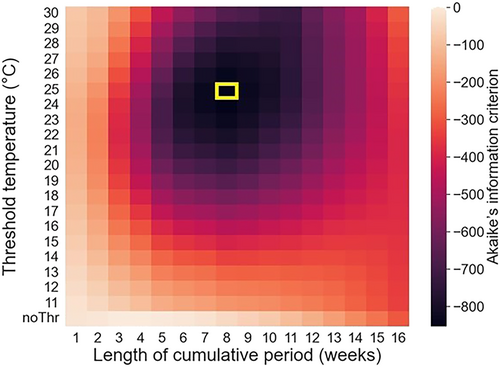
Changes in Akaike's information criterion (AIC) of the linear model for the average cumulative thermal load (TL) changing the length of the cumulative period in weeks and the threshold temperature.
Note: TL, cumulative value of the maximum temperatures that exceeded the threshold temperature for the cumulative period before the end of performance testing; noThr, TL calculated without threshold temperature. The AIC of the model without TL was set to 0. The area framed in yellow is the minimum AIC.
Some information about high-heat environment indicators in purebred Duroc pigs has been previously reported. Ogawa et al. (2022) reported a daily average temperature threshold of 24.2°C and a 50-day period before reaching 105 kg. Fragomeni et al. (2016) reported a temperature threshold value of 23.7°C (the daily maximum THI was converted to the temperature at 50% relative humidity) and a 30-day period before the end of performance testing. Compared with previous studies, the difference in the threshold temperature was approximately 1°C; however, the period was considerably longer.
The distribution of TL by farm in 2022 is shown in Figure 2, and the basic statistics of TL and E(D105|TL) in 2022 are shown in Table 2. The duration and intensity of TL differed across farms, increasing around June on farm A, approximately 2 months later than that on the other farms, and decreasing around November on all farms. The intensity of TL differed considerably by farm region. Farm A is located in the northern part of Japan (Hokkaido Prefecture), and two other farms are located in the central part of Japan (Honshu Island). values changed owing to and TL. The TL calculated from the weather records of 2022 for each farm suggested that shipment may have been delayed by up to 1.6, 7.5, and 5.7 days from TL = 0 (corresponding to −8.0, −33.4, and −27.7 g/days in ADG) because of TL on farms A, B, and C, respectively. Notably, Ogawa et al. (2022) investigated the effect of the daily average temperature on D105 in 2020 and reported a possible shipping delay of up to 9 days on a farm south of the farms investigated in the present study.
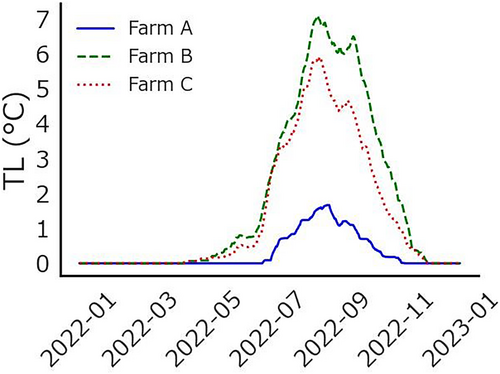
Behavior of average cumulative thermal load (TL) in 2022 for each farm (only the farms with pig records are shown).
Note: TL, average cumulative value of the maximum temperatures that exceeded 25°C in the on-farm estimated weather records for the 8 weeks before the end of performance testing. Farm A, Kita-Hiroshima City, Hokkaido Prefecture, 43.0°N; Farm B, Nagaoka City, Niigata Prefecture, 37.4°N; and Farm C, Shibukawa City, Gumma Prefecture, 36.5°N.
| TL (°C) | (age in days) | |||||
|---|---|---|---|---|---|---|
| Farm | A | B | C | A | B | C |
| Mean | 0.3 | 1.8 | 1.4 | 145.7 | 151.5 | 144.8 |
| SD | 0.5 | 2.4 | 1.9 | 5.9 | 4.6 | 4.3 |
| Minimum (min) | 0.0 | 0.0 | 0.0 | 139.7 | 143.3 | 139.1 |
| Maximum (max) | 1.7 | 7.1 | 5.9 | 156.1 | 159.7 | 152.0 |
| Calculated average daily gain (ADG) (g/days) | ||||||
| TL condition [calculation formula] | A | B | C | |||
| Mean [] | 720.7 | 693.1 | 725.1 | |||
| Min [] | 722.1 | 701.5 | 731.7 | |||
| Max [] | 714.1 | 668.2 | 704.0 | |||
| Effect of max TL [] | −8.0 | −33.4 | −27.7 | |||
| Calculated (age in days) | ||||||
| TL condition [calculation formula] | A | B | C | |||
| Min [] | 145.4 | 149.7 | 143.5 | |||
| Max [ | 147.0 | 157.1 | 149.2 | |||
| Expected shipment delay (days) | ||||||
| Calculation formula | A | B | C | |||
| 1.6 | 7.5 | 5.7 | ||||
- Note: Farm A, Kita-Hiroshima City, Hokkaido Prefecture, 43.0°N; Farm B, Nagaoka City, Niigata Prefecture, 37.4°N; and Farm C, Shibukawa City, Gumma Prefecture, 36.5°N (Only the farms with pig records are shown); TL, average cumulative value of the maximum temperatures which exceeded 25°C in the on-farm estimated weather records for the 8 weeks before the end of performance testing; , the solution of the partial regression coefficient of TL (−4.7).
Records from 2001 to 2022 were used in the present study. A total of 22,043 records had a TL of 0, and 32,707 records had a TL > 0. The records with a TL > 0 accounted for approximately 60%, with an average TL value of 2.0. This result suggests that many pigs in Japan may have already experienced delayed shipment because of reduced ADG under high-heat environments. Therefore, improving heat tolerance in pigs is an urgent issue.
3.3 Estimates of variance components
The estimates of variance components are presented in Table 3. All estimates of , , and significantly differed from 0 (95% confidence interval). Estimated total genetic variance () ranged within 298 (TL of 2.6) to 1376 (TL of 8) (g/day)2.
| Parameter/item | Genetic variance | Error variance | Heritability and genetic correlation | ||||||
|---|---|---|---|---|---|---|---|---|---|
| Parameter | |||||||||
| Estimated values | 537 | −93 | 36 | 505 | −0.67 | ||||
| SE | 18 | 5 | 2 | 8 | 0.02 | ||||
| Parameter | |||||||||
| TL | 0 | 1 | 2 | 3 | 4 | 5 | 6 | 7 | 8 |
| Estimated values | 537 | 387 | 309 | 305 | 373 | 514 | 729 | 1016 | 1376 |
| SE | 18 | 14 | 13 | 14 | 17 | 24 | 36 | 52 | 73 |
| Parameter | |||||||||
| TL | 0 | 1 | 2 | 3 | 4 | 5 | 6 | 7 | 8 |
| Estimated values | 0.52 | 0.43 | 0.38 | 0.38 | 0.42 | 0.50 | 0.59 | 0.67 | 0.73 |
| SE | 0.01 | 0.01 | 0.01 | 0.01 | 0.01 | 0.01 | 0.01 | 0.01 | 0.01 |
- Note: TL, average cumulative thermal load (°C); , additive genetic variance for ; , additive genetic variance for ; , additive genetic covariance for and ; ; , heritability at TL; , random error variance; , genetic correlation for and .
The estimates of the heritability of the ADG in purebred Duroc pigs are moderate, ranging from 0.32 to 0.50 (Do et al., 2013; Ogawa et al., 2022, 2023; Suzuki et al., 2005). The change in heritability estimated using RNAM under varying TL conditions ranged from 0.38 (TL of 2.6) to 0.73 (TL of 8). For TL values of 0 to 2.6, estimated heritability decreased with increasing TL values. This was because the decrease caused by the negative genetic covariance of and in response to TL () exceeded the increase in the genetic variance of in response to TL (). For TL values > 2.6, heritability estimates increased with TL values. This was because the increase in genetic variance of in response to TL was greater than the decrease in additive genetic covariance in response to TL. Similar to the present study, Fragomeni et al. (2016) reported that the estimated heritability varied with high-heat environmental indicator values in a U-shape, with higher heritability at higher indicator values. They attributed this result to the fact that the genetic ability at high-heat environments has not been selected for under directional selection; thus, the additive genetic variance is retaining. As the expression of the effect is dependent on TL conditions, the results suggest the feasibility of genetically improving heat tolerance using in the evaluation model. However, the estimated genetic correlation between and was negative (). Effective and simultaneous improvement of both and would be challenging. Similarly, a negative genetic correlation was also estimated in a previous study involving reaction-norm sire model analysis of crossbred pig carcass weight (Zumbach et al., 2008a).
The estimated genetic correlations for ADG under different TL conditions are shown in Figure 3. Genetic correlation became lower as the difference between the two TL values increased. The minimum genetic correlation was −0.2 for the minimum (0) and maximum (8) TL values. Mulder et al. (2006) suggested that G × E should be considered in selection when the genetic correlation between different environments is less than 0.6. In the present study, the estimated genetic correlations were below this value when the differences between TLs were large. Regarding the genetic correlation between different indicators of high-heat environments, Usala et al. (2021) reported a case in which the genetic correlation was less than 0.6 for pig carcass ADG.
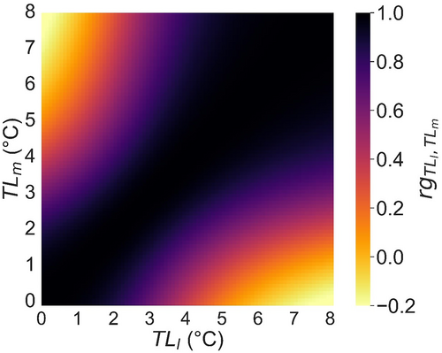
Genetic correlation () for average daily gain (g/day) under different TL conditions (between and values) estimated using the reaction norm animal model.
Note: TL, average cumulative thermal load (°C); the upper limit of TL is the maximum value of the dataset.
3.4 Estimated breeding value
The and of pigs born in 2022 ranged from −10.7 to 72.8 and from −13.0 to 0.22, respectively. The changes in DevADG with TL in pigs born in 2022 are shown in Figure 4. The population means of ADG (thick black line) decreased with increasing TLs. Low- pigs (blue dotted line) tended to have higher DevADGs than those of high- pigs (red line) at TL = 0; however, DevADGs decreased considerably with increasing TL. In contrast, high- pigs (red line) tended to have lower DevADGs than those of low- pigs at TL = 0; however, their declining rates with increasing TL were slower than those of low- pigs. The change in the ranking of pigs with varying TLs suggests the need to evaluate EBV using a model that effectively considers G × E. Simms (2000) stated that the slope term quantifies tolerance in RNM. Similarly, in the present study, heat tolerance was also expressed by the slope term in the RNAM. Therefore, to genetically improve heat tolerance, it is crucial to evaluate in RNAM and consider it in selection.
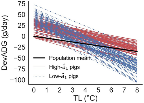
Changes in average daily gain deviation from the population mean (DevADG) with TL in pigs born in 2022.
Note: TL, average cumulative thermal load (°C); population mean vary with , calculated by ; high- and low- pigs were selected using the value of from 364 male pigs born in 2022; ; , estimated breeding value of kth pig under condition, calculated by ; , the solution of the partial regression coefficient of TL via reaction-norm animal model (RNAM); , intercept term of EBV in RNAM (g/day); , slope term of EBV in RNAM (g/day). The upper limit of TL is the maximum value of the data set.
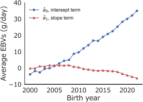
The trends in EBVs by birth year are shown in Figure 5. The values of exhibited an increasing trend, whereas showed a decreasing trend. [Correction added on 12 June 2024, after first online publication: Preceding sentence has been amended for correctness.] However, there is variation in the values for pigs born in 2022, suggesting that genetically superior heat-tolerant pigs may still be present in the current Duroc pig population. The Intergovernmental Panel on Climate Change (2022) predicts that global warming will worsen. As global warming becomes more severe and economic losses increase, heat-tolerant selection in pigs is expected to become more important. To prevent economic losses and secure heat-tolerant pig genetic resources, incorporating genetic evaluation for heat tolerance into breeding programs is necessary.
3.5 Future perspective
The present study focused on purebred Duroc pigs; however, other breeds such as Landrace and Large White should also be analyzed. As modern commercial pork production is largely supported by a crossbreeding system, the utilization of crossbred pig records also remains a future challenge. Furthermore, genetic relationships between other production or reproductive traits should be clarified for comprehensive breeding (e.g., Bloemhof et al., 2013; Fragomeni et al., 2016; Freitas et al., 2021, 2023; Sevillano et al., 2016; Tiezzi et al., 2020; Usala et al., 2021; Zumbach et al., 2008a).
ACKNOWLEDGMENTS
This research forms part of the results of a project funded by the Japan Central Racing Association for the Promotion of Livestock Production, “Development of Global Warming-Adaptive Swine Breeding Methods Project.”
The authors would like to thank Mr. Kotaro Akachi, President of Akachi Genetics, Inc., Mr. Kazuyuki Tashima, and other members of Global Pig Farms, Inc., and related farms for their cooperation in collecting data for this study.
CONFLICT OF INTEREST STATEMENT
The authors declare that they have no conflict of interest.
ETHICS STATEMENT
The study did not require approval from the Animal Care and Use Committee as the data were obtained from an existing database maintained by a private breeding company.
Open Research
DATA AVAILABILITY STATEMENT
The pig records used in this study are properties of the industry partners that contributed to the study and, therefore, are not available owing to their commercial sensitivity. Kindly contact Agro-Meteorological Grid Square Data (https://amu.rd.naro.go.jp/) for information on using weather records.


