Partial moment volatility indices

3.1 Data collection

Historical prices of SPX call and put options were based on closing quotes of SPX from 4 January 1996 to 30 August 2013 obtained from OptionMetrics. Data include the highest closing bid and ask quotes for each SPX option, and Black-Scholes implied volatilities based on the average of best bid and ask. Using the standard approach of the Chicago Board Options exchange (CBOE) with the option price approximated by the average of best bid and ask.

US one-month and three-month Treasury-bill yields were used as risk-free interest rates, after adjusting for dividend yields. Treasury-bill and dividend yields are obtained from the Federal Reserve Bulletin and Option Metrics, respectively. For SPX option with the maturity shorter (longer) than either of the two Treasury-bill maturities, the risk-free rate is approximated by the dividend-adjusted one-month (three-month) yield.

Daily quotes of VIX are obtained from both OptionMetrics and CBOE VIX Historical Price Data7 to ensure the completeness of the data.

Common data filters are applied. SPX options with maturities less than 7 and greater than 81 days are excluded, to avoid any market microstructure impacts, liquidity issues and price effects near contract expiration (Figlewski, 2010). Options with bid prices below $0.05 are eliminated, along with any put (call) options with strike prices lower (higher) than that of the first two consecutive puts (calls) with zero bid prices. At- and out-of-the-money options are also excluded, along with options with Black-Scholes implied volatilities below 0 or above 1.

3.2 Methodology

The basic form of the state-preference pricing equation is:

(3)

summing over all possible states {1,…, S}. P_t is the price of some asset at time t, Φ_s,t + 1 is the state price, and d_s,t + 1 is the pay-off of this asset at state s and time t + 1. BEX2 is calculated with a similar process to the theoretical derivation of VIX, by replicating the fair value of future variance, with BEX its squared-root. BUX can be obtained similarly.

BEX² represents a financial asset that pays a dollar amount of (ln(K_s/S₀))² at future date T, for every future index level K_s and spot price level S₀ if K_s ≤ S₀, or $0 otherwise. Following the state-preference pricing approach, BEX² can be obtained as:

(4)

Here S₀ is the current SPX level, K_s is the sth option with strike K_s, T is the time to maturity,8 and Φ_s is state price (or equivalently the risk-neutral probability) at strike price K_s. Here T is set to be exactly 30 calendar days (or equivalently, 22 trading days). Comparison of equations 3 and 4 reveals that the pay-off for each state is defined to be

(5)

As discussed in the previous section, we assume an industry standard zero mean assumption for short-term SPX returns. We also consider the nonzero mean counterparts, where Treasury-bill yields and the realised mean return of SPX over the most recent thirty trading days are adopted. Results are qualitatively the same.

Likewise, BUX² is obtained by changing the indicator function such that BUX² only pays out a positive amount if K_s > S₀, or $0 otherwise:

(6)

Having defined the pay-off in each state, the next task is to estimate the state prices. Liu and O'Neill (2015) developed an alternative volatility index SVX as a forecast for market realised volatility using the state-preference pricing approach of Breeden and Litzenberger (1978) with Black-Scholes analytic second derivatives. They demonstrate that SVX behaves like the current market volatility barometer VIX and outperforms VIX in forecasting the future market realised volatility. In this study, we use the same state prices obtained from constructing SVX as the state price inputs to construct BEX and BUX. The state prices are computed as:

(7)

where K_i < K_i + 1 and

(8)

where q is the dividend yield. The key input is the volatility parameter σ, estimated as the average Black-Scholes implied volatility from two ATM call and put options from two maturities that are closest to a 30-day period. Implied volatility is generally found to have better information content other measures of historic volatility (Brace and Hodgson, 2009).9

To obtain a smoother state price density, states range from 0.1 to 9,999 in 0.10 increments. A state of 200 indicates the SPX will be at 200 after 1 month. Given that SPX fluctuates from 598.48 to 1709.67 from 1996 to 2013, our choice covers a much bigger range than that of VIX. Because each state price represents an interval from K_i to K_i+1, we need to modify the state pay-offs to get to the centre of the 10-cent interval.

(9)

(10)

Summing all products of the state pay-off and the state price, we obtain the BEX² and BUX². BEX and BUX are obtained by taking the square root of these measures.

3.3 Description of indices

In this section, we examine the historical behaviour of BEX and BUX. Table 1 reports the summary statistics on levels and logarithmic returns of BEX, BUX, VIX and the corresponding subsequent 30-day realised LPM and UPM volatilities in SPX market and . Logarithmic returns are defined as, for example, ∆BEX_t = ln(BEX_t/BEX_t−1). Each series has 4445 daily observations from 4 January 1996 to 30 August 2013. All entries are represented in percentage volatility points. As we have set h = 0 in BEX and BUX, we use the zero mean assumption in realised LPM and UPM variance calculation for a direct comparison. Two ex post LPM and UPM realised volatility estimates are estimated, as shown in equations 11 and 12, respectively.

(11)

(12)

Table 1. Summary statistics of BEX, BUX, VIX, LPM and UPM realised SPX return volatilities

Moments	BEX	BUX	VIX			ΔBEX	ΔBUX	ΔVIX
Mean	15.51	12.34	21.74	12.51	12.79	0.00	0.00	0.00	0.00	0.00
Median	14.61	11.62	20.31	10.66	10.94	0.00	0.00	0.00	0.00	0.00
Maximum	60.16	47.85	80.86	68.20	60.27	0.53	0.47	0.50	0.94	0.83
Minimum	6.68	5.32	9.89	1.23	3.43	−0.51	−0.55	−0.35	−1.05	−0.71
Std. Dev.	6.23	4.96	8.48	8.30	7.05	0.07	0.07	0.06	0.11	0.09
Skewness	1.94	1.94	1.94	2.57	2.59	0.43	0.43	0.59	−0.25	0.55
Kurtosis	9.64	9.64	9.63	13.24	13.30	6.71	7.11	6.78	23.29	16.20

• This table reports the sample mean, median, maximum, minimum, standard deviation, skewness and kurtosis on the levels and logarithmic returns of the lower partial moment (LPM) volatility index BEX, the upper partial moment (UPM) volatility index BUX, the CBOE volatility index VIX, the 30-day LPM and UPM realised volatilities with calendar days convention and , respectively. The logarithmic return is defined as, for example, ∆BEX_t = ln(BEX_t/BEX_t−1). Each series has 4445 daily observations from 4 January 1996 to 30 August 2013. All entries are represented in percentage volatility points.

In Table 1, the sample means of BEX and BUX are 15.51 and 12.34, respectively. As expected, the sample means, medians, maximums and standard deviations of BEX and BUX are smaller than those of VIX, as the measures only describe a portion of the return distribution

The sample mean of BUX is similar to at 12.79, although the standard deviation of BUX is smaller than the realised counterpart. In comparison, the sample mean of BEX is much higher than , with a difference of 3. This suggests index options traders are more risk averse and pay a premium for extreme losses or ‘Black swan’ events, consistent with the findings in Bates (1991) and Rubinstein (1994).10

For logarithmic daily changes, all sample means are approximately zero. Standard deviations, absolute maximums and minimums of ∆BEX, ∆BUX and ∆VIX are all smaller than their ex post realised counterparts. This suggests that while risk-neutral moments over-estimate the ex post measures on average, they appear less volatile in daily changes and do not capture them in extreme market conditions.

Table 2 reports the cross-correlations between BEX, BUX, VIX and 30-day forward LPM and UPM realised SPX return volatilities. Although based on different methodologies, BEX, BUX and VIX are highly positively correlated in both levels and logarithmic daily changes, and all three correlate with ex post realised measures. However, these correlations become negligible in the daily changes.

Table 2. Cross-correlations of BEX, BUX, VIX and 30-day forward-looking LPM and UPM realised SPX return volatilities

Correlation	BEX	BUX	VIX			ΔBEX	ΔBUX	ΔVIX
BEX	1.00	0.99	0.99	0.64	0.82
BUX	0.99	1.00	0.99	0.64	0.82
VIX	0.99	0.99	1.00	0.63	0.81
	0.64	0.64	0.63	1.00	0.80
	0.82	0.82	0.81	0.80	1.00
ΔBEX						1.00	0.99	0.90	−0.37	0.31
ΔBUX						0.99	1.00	0.90	−0.38	0.31
ΔVIX						0.90	0.90	1.00	−0.39	0.32
						−0.37	−0.38	−0.39	1.00	−0.15
						0.31	0.31	0.32	−0.15	1.00

• This table reports cross-correlations on the levels and logarithmic returns of the lower partial moment (LPM) volatility index BEX, the upper partial moment (UPM) volatility index BUX, the CBOE volatility index VIX, the 30-day LPM and UPM realised volatilities with calendar days convention and , respectively. The logarithmic return is defined as, for example, ∆BEX_t = ln(BEX_t/BEX_t−1). Each series has 4445 daily observations from 4 January 1996 to 30 August 2013.

Figure 1 shows daily closing levels of BEX, BUX, VIX and the scaled S&P 500 index from 6 January 1996 to 30 August 2013. It is clear that BEX and BUX follow VIX, especially during the GFC. BEX is invariably higher than BUX. The difference between BEX and BUX appears to increase when the market is moving downwards particularly around the mid-2003 and post-GFC, and becomes almost negligible when the market is moving upwards.

4.1 Forecasting partial moment volatilities

The VIX is a measure of ex ante 30-day expected volatility of the S&P 500 index (CBOE, 2009). VIX does not, however, describe the proportion of upside potential versus downside threat. To solve this problem, we construct BEX (BUX) as a predictor of the ex ante 30-day expected LPM (UPM) volatility and expect they provide a better forecast in the corresponding partial moment volatility than VIX.

To test this proposition, we regress the subsequent realised LPM (UPM) volatilities in calendar days with BEX (BUX) and VIX, respectively. Our tests are in the following forms:

(13)

Hypotheses are tested using these regressions. First, if BEX and VIX contain some information about future realised LPM volatility, then the slope coefficients should be nonzero. Second, if BEX and VIX are unbiased forecasts of future realised LPM volatility, one should expect an intercept of zero and slope coefficients not significantly different from 1. We report the ordinary least-squares estimates in Table 3. The covariance matrix is computed according to Newey and West (1994) to correct for any potential serial correlations in the error terms.

Table 3. Regression results of BEX, BUX and VIX against 30-day forward-looking LPM and UPM realised SPX return volatilities

Panel A		Coefficient	Std. error	t-Statistics	Prob.	Adj. R2	Wald test
	BEX	0.852	0.069	12.300	0.0000		0.0132
	Intercept	−0.726	0.965	−0.752	0.452	40.9%
	VIX	0.621	0.050	12.519	0.0000		0.0000
	Intercept	−1.011	0.973	−1.039	0.299	40.2%

Panel B
	BUX	1.164	0.066	17.527	0.0000		0.0281
	Intercept	−1.596	0.725	−2.199	0.0279	67.1%
	VIX	0.673	0.038	17.650	0.0000		0.0000
	Intercept	−1.859	0.733	−2.538	0.011	65.6%

• This table presents regression results of the lower partial moment (LPM) volatility index BEX, the upper partial moment (UPM) volatility index BUX and the CBOE volatility index VIX against the 30-day LPM and UPM realised volatilities with calendar days convention and , respectively. There are 4445 daily observations from 4 January 1996 to 30 August 2013 in each series. The heteroskedasticity-consistent standard errors and covariance matrix are computed according to Newey and West (1994) with the lag truncation of 8. Regressions equations are presented in equation 13. All volatility estimates calculate the realised volatility using monthly logarithmic returns. The last column on the right reports the F-statistics in the Wald Test, which is to test whether the slope coefficient is significantly different from 1. The lower the number, the higher the chance of being significantly different from 1.

Panel A reports the regression results of BEX and VIX against . The estimate of intercept α₀ is −0.726 and is not statistically significantly against a null of α₀ = 0 at the 5 percent level. Similarly, for VIX, the estimate of β₀ is −1.011 and also not statistically significantly different from 0.

For the slope coefficients, the estimate of α₁ is 0.852 and is statistically significant against a null of α₁ = 0. This indicates that BEX contains information about future realised LPM volatility. In comparison, the estimate of β₁ from the regression of and VIX is 0.621 with a standard error of 0.05. This is statistically significant against a null of β₁ = 0. We also run the Wald test, rejecting the null hypothesis at the 5 percent level for BEX and at all levels for VIX. The slope coefficient of VIX is more likely to be statistically different from 1 than that of BEX. The adjusted R² of BEX model is 40.9 percent, being 0.7 percent higher than the VIX model. We conclude that BEX is a better predictor of future realised LPM volatility.

We also test hypotheses related to BUX and VIX. First, if BUX and VIX contain some information about future realised UPM volatility, then slope coefficients in equation 13 should be nonzero. If BUX and VIX are unbiased forecasts of future realised UPM volatility, one should expect an intercept of zero and slope not significantly different from 1.

Panel B reports the regression results of BUX and VIX against . The estimate of intercept γ₀ is −1.596 which is statistically significant against a null of γ₀ = 0 at the 5 percent level. Similarly, the estimate of λ₀ is −1.859 and also statistically significantly different from 0. Both BUX and VIX provide biased forecasts, but this should not be problematic if the magnitude of the bias is constant.

For the slope coefficients, the estimate of γ₁ is 1.164, being statistically significant against a null of γ₁ = 0. In comparison, the estimate of λ₁ from the regression of LPM and VIX is 0.673 with a standard error of 0.038. Again, the Wald test statistics show that we reject the null hypothesis at the 5 percent level.

Table 3 also shows that while BEX overestimates UPM volatility, BUX does the opposite, implying that SPX option traders tend to underestimate upside potential and overestimate the downside threats. This is consistent with findings in Bakshi et al. (2003) that the market is risk-neutrally left-skewed. The adjusted R² of the BUX model is 67.1 percent, being 1.5 percent higher than the VIX model. We conclude that BUX is a less unbiased forecast with greater predictive power for future realised UPM volatility.

4.2 Explaining contemporaneous changes in daily market returns

There is a well-documented negative relation between expected returns and changes of volatility (Campbell et al., 1997). Increases in volatility tend to lower returns, with volatility considered a negative signal in portfolio performance. We split volatility into downside and an upside components and examine their relations with the contemporaneous returns, estimating regressions in the following forms:

(14)

where the daily change is defined as ∆SPX_t = ln(SPX_t/SPX_t−1) and 11

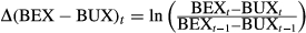
To examine relationships among BEX, BUX and market returns, we need to include both BEX and BUX as explanatory variables. To overcome the problem with multicollinearity between BEX and BUX, we create a variable that takes the difference of BEX and BUX on each trading day. It is well documented that empirical returns are asymmetric (Bates, 1991 and Rubinstein, 1994). Subtracting BEX_t by BUX_t describes how much more deviation is expected in the downside than the upside from the options market. A positive ∆(BEX − BUX)_t shows that the difference between the downside and upside risk becomes larger with BEX_t − BUX_t > BEX_t−1 − BUX_t−1, meaning more downside losses versus upside gains. This definition allows us to extract the risky component of volatility.

Two hypotheses can be tested using regressions in equation 14. First, if there is a negative relation between returns and changes of volatility, the slope coefficient β₁ should be negative, consistent with results in the literature. Second, given that ∆(BEX − BUX)_t measures variation between the difference in downside and upside volatilities, we expect a negative relation with the market return, with α₁ < 0.

Table 4 reports ordinary least-squares results. The covariance matrix is computed according to Newey and West (1994) to correct for potential serial correlations in errors.

Table 4. Regression results of ΔSPX_t against Δ(BEX – BUX)_t and ΔVIX_t

Panel A	ΔSPXt	Coefficient	Std. error	t-Statistics	Prob.	Adj. R2
	Δ(BEX – BUX)t	−0.132	0.005	−24.607	0.0000
	Intercept	0.0002	0.0001	1.890	0.0588	52.3%

Panel B	ΔSPXt
		−0.154	0.006	−26.837	0.0000
	Intercept	0.0002	0.0001	1.912	0.056	56.4%

• This table presents the regression results of the daily logarithmic change of the lower partial moment (LPM) volatility index BEX and the upper partial moment (UPM) volatility index BUX against the daily logarithmic return of S&P 500 index. The daily changes are defined as, ΔSPX_t = ln (SPX_t – SPX_t−1) and . There are 4445 daily observations from 5 January 1996 to 30 August 2013 in each series. The heteroskedasticity-consistent standard errors and covariance matrix are computed according to Newey and West (1994) with the lag truncation of 8. Regression equations are presented in equation 14.

Panel A reports the results for ∆(BEX − BUX)_t against ∆SPX_t. The estimate of α₀ is 0.0002 and is not significantly different from 0 at all levels. The estimate of α₁ is −0.132 with a standard error of 0.005, and we cannot reject a null of α₁ < 0 at any level. Similar results can be found in the bottom panel for ∆VIX_t with intercept not significantly different from 0 and slope −0.154 with a standard error 0.006.

Although both slope coefficients are negative, more insight is provided by the first regression. While the negative β₁ from the second regression is consistent with prior literature evidencing a negative relation between changes in volatility and market returns, the negative α₁ emphasises that the negative relation between risk and return comes from the downside. The volatility feedback effect states that an anticipated increase in volatility leads to an immediate price drop. By extracting the risky component of volatility, we show that when downside volatility exceeds upside volatility, this excess contributes to the decline in returns.

4.3 Investor fear gauge: BEX or VIX

VIX is well-known as the investors’ fear gauge in that it responds more to negative changes in index returns than the positive changes (Whaley, 2009). BEX is constructed as the forecast of LPM volatility focusing on negative future returns, so might be better qualified as a fear barometer. This is assessed by estimating regressions as follows:

(15)

where daily change is defined as, for example, ∆BEX_t = ln(BEX_t/BEX_t−1). describes the rate of change of SPX conditional on whether it is a negative return,  = min(0, ∆SPX_t).

Three hypotheses are tested. First, if the rate of change in BEX and VIX is related to daily market returns, then the slope coefficients α₁ and β₁ should be negative. Second, coefficients α₂ and β₂ should also be negative to reflect an asymmetric response to market declines. Third, if this relationship is unbiased, then intercepts should be zero.

Table 5 reports ordinary least-squares results with the covariance matrix computed according to Newey and West (1994) with a lag truncation of 8.

Table 5. Regression results of ∆BEX_t and ∆VIX_t against the rate of change and conditional rate of change of S&P 500 index

Panel A	ΔBEXt	Coefficient	Std. error	t-Statistics	Prob.	Adj. R2
	ΔSPXt	−3.541	0.161	−22.041	0.000
		−0.811	0.263	−3.087	0.002
	Intercept	−0.003	0.001	−2.412	0.016	52.6%

Panel B
	ΔSPXt	−3.187	0.146	−21.785	0.000
		−0.885	0.249	−3.554	0.000
	Intercept	−0.003	0.001	−3.040	0.0002	56.9%

• This table presents the regression results of the daily logarithmic change of the lower partial moment (LPM) volatility index BEX and the volatility index VIX against the daily logarithmic return and conditional return of S&P 500 index. The daily change is estimated as ∆SPX_t = ln(SPX_t/SPX_t−1). The conditional rate of change of S&P 500 index, depending on whether it is a negative return, is estimated as  = min(0, ∆SPX_t). The heteroskedasticity-consistent standard errors and covariance matrix are computed according to Newey and West (1994) with the lag truncation of 8. Regression equations are presented in equation 15.

Panel A presents results for BEX, with α₁ estimated at −3.541 with a standard error of 0.161. This is statistically significant against a null of α₁ = 0 at all levels. The estimate of α₂ is −0.811 with a standard error of 0.263 and is also statistically significant against a null of α₂ = 0 at all levels. The intercept is −0.003 with a standard error of 0.001, being statistically significant against a null of α₀ = 0 at the 5 percent level. This reflects not only the inverse relationship between movements in BEX and movements in the SPX market, but also the asymmetry.

The bottom panel B presents the result of VIX, confirming Whaley (2009). However, the p-value for intercept term β₀ is also statistically significant against a null of 0. That is, the relationship between these contemporaneous changes tends to be biased.

These coefficients can be interpreted as follows. If the market goes up by 100 basis points, BEX and VIX will likely fall by an amount of:

On the other hand, if the market drops by 100 basis points, BEX and VIX will likely rise by an amount of:

That is, when there is a drop in the market, a larger response is found in BEX than VIX. BEX rises by an extra 27 basis points for every 100 basis points drop in SPX. We conclude that BEX may be more qualified as the barometer of investors’ fear for downside threats than VIX.