Stochastic Joint Inversion of Seismic and Controlled-Source Electromagnetic Data
ABSTRACT
Stochastic inversion approaches provide a valuable framework for geophysical applications due to their ability to explore multiple plausible models rather than offering a single deterministic solution. In this paper, we introduce a probabilistic joint inversion framework combining the very fast simulated annealing optimization technique with generalized fuzzy c-means clustering for coupling of model parameters. Since very fast simulated annealing requires extensive computational resources to converge when dealing with a large number of inversion parameters, we employ sparse parameterization, where models are sampled at sparse nodes and interpolated back to the modelling grid for forward computations. By executing multiple independent inversion chains with varying initial models, our method effectively samples the model space, thereby providing insights into model variability. We demonstrate our joint inversion methodology through numerical experiments using synthetic seismic traveltime and controlled-source electromagnetic datasets derived from the SEAM Phase I model. The results illustrate that the presented approach offers a practical compromise between computational efficiency and the ability to approximate model uncertainties, making it suitable as an alternative for realistic larger-scale joint inversion purposes.
1 Introduction
- 1. Although a joint inversion is likely to narrow down the number of possible solutions, the inversion problem remains non-unique and the constructed model may still not be a true representation of the subsurface.
- 2. In realistic models, petrophysical relationship(s) among different model parameters could be complicated, which requires an efficient coupling strategy in the joint inversion algorithm.
The first challenge becomes particularly important when a deterministic method is used for joint inversion, as it typically produces a single ‘best-fit’ model without conveying any information about variability in the solution space. In contrast, probabilistic global optimization methods such as very fast simulated annealing (VFSA) used in this paper, although not designed to sample the full posterior distribution like Markov chain Monte Carlo (MCMC), operate within a stochastic framework that enables limited exploration of the model space. By running multiple inversion chains from different initial conditions, VFSA can yield an ensemble of plausible models that fit the data. While this ensemble does not constitute a statistically rigorous posterior sample, it can still reveal meaningful variability in model parameters and provide qualitative insights into solution stability. In this article, we use the term uncertainty in a qualified sense to refer to this ensemble-based variability, acknowledging that it offers only an approximate view of the inherent non-uniqueness of the geophysical inverse problem.
Some previous works in the context of probabilistic joint inversion have used Monte Carlo (MC) method (Bosch and McGaughey 2001; Chen et al. 2004; Bosch et al. 2006; Jardani and Revil 2009; Shen et al. 2013), co-kriging method (Shamsipour et al. 2012), MCMC method (Rosas-Carbajal et al. 2014; Wéber 2018), trans-dimensional MCMC (Blatter et al. 2019), and VFSA method (Kaikkonen and Sharma 1998; Yang et al. 2002; Hertrich and Yaramanci 2002; Santos et al. 2006).
Among the approaches listed, MC methods are considered the most statistically rigorous, as they aim to produce independent samples drawn directly from the target posterior distribution. Model proposals are generated randomly across the parameter space and accepted or rejected based on the Metropolis–Hastings criterion (Metropolis et al. 1953). While MC sampling provides a high-fidelity estimate of the posterior probability distribution (PPD), it is computationally intensive and often impractical for high-dimensional or computationally expensive forward models (Sen and Stoffa 2013).
MCMC methods improve computational feasibility by constructing a Markov chain whose stationary distribution is the posterior. Each new model is generated conditionally based on the current model, enabling the chain to concentrate sampling in regions of high posterior probability. Although this results in dependent samples, the method is more efficient than standard MC for large-scale inverse problems. Sen and Stoffa (1996) review a range of such sampling-based approaches and show that with suitable modifications, optimization algorithms like VFSA can approximate features of the PPD at substantially lower computational cost. VFSA, originally developed as a global optimizer, uses a cooling schedule combined with the Metropolis–Hastings acceptance rule. When applied with multiple runs or at a fixed temperature, VFSA can yield ensembles that approximate posterior-like distributions (Roy, Sen, Blankenship, et al. 2005; Roy, Sen, McIntosh, et al. 2005), offering a practical alternative for exploring model variability in joint inversion frameworks.
There are two main differences between MCMC and VFSA as the latter uses a temperature-dependent Cauchy distribution to draw the proposal model, which tends to narrow down the proposal to the previous state as the temperature decreases. Moreover, the probability of accepting a ‘bad’ model also decreases over the number of iterations and becomes sufficiently low near the global minimum. The PPD derived from a single chain of VFSA is inherently biased towards the global minimum; therefore, multiple chains of VFSA are needed to get many plausible models for uncertainty quantification. Although the PPD estimated through rigorous sampling methods is more accurate, the same obtained through the VFSA does provide a ‘sweet spot’ between affordability and accuracy.
The second challenge, that is, effective coupling of model parameters has mostly been discussed in the context of deterministic joint inversion, which can be categorized as (1) structure-based coupling (Haber and Oldenburg 1997; Gallardo and Meju 2004) and (2) petrophysical coupling (Koketsu and Nakagawa 2002; Jegen et al. 2009). A detailed review of different approaches for parameter coupling can be found in Colombo and Rovetta (2018). In this paper, we use a guided fuzzy c-means (FCM) clustering developed by Sun and Li (2012), which is a generalized version of the the method proposed by Lelièvre et al. (2012) and has been effectively used in deterministic joint inversion in geoscience (Sun and Li 2016a, 2016b; Darijani et al. 2020).
In this paper, we introduce a probabilistic joint inversion approach for multi-physics data integration, utilizing the VFSA algorithm combined with a generalized FCM clustering method (Dunn 1973; Bezdek 1981). Given that a large number of inversion parameters would typically necessitate an impractically high number of VFSA iterations for convergence, we employ a sparse parameterization strategy to randomly distribute inversion points across the model space. We provide a detailed discussion of the VFSA and FCM algorithms, explaining our rationale for their selection in the joint inversion framework. To validate the proposed algorithm, we present numerical experiments on the joint inversion of first-arrival seismic traveltime and controlled-source electromagnetic data for a 2D slice of the SEAM Phase I model, focusing on computing mean models and associated uncertainties.
2 Methods
2.1 Sparse Parameterization
To ensure that very fast simulated annealing (VFSA) can reliably converge within realistic computational budgets, we reduce the number of free parameters in the inverse problem using a sparse parameterization strategy. The sparse parameterization strategy applied in this study is illustrated in Figure 1, which displays four panels highlighting each step of the workflow. Panel a shows the model at iteration on the full computational grid, including a blue water layer at the top and a red anomaly in the subsurface. Rather than assigning an inversion parameter to every cell, a set of control points (150) is defined in panel b to represent the model with far fewer parameters. These points are placed more densely in regions of anticipated complexity, such as the anomalous zone, and each carries a single value later interpolated across the entire domain. This approach substantially reduces the dimensionality of the inverse problem while maintaining the flexibility needed to capture critical structural variations. This shows that one can adaptively distribute control points if one expects a more complex model in certain locations. Panel c demonstrates how a model is updated during a VFSA iteration. Panel d then shows the updated velocity model after re-interpolation onto the full simulation mesh, reflecting new parameter values below the water layer. Subsequent tests in this paper adopt a simpler random distribution of control points and use linear radial-basis functions for interpolation.

One important concern in sparse parameterization is how to choose the number of control points. This choice is somewhat ad hoc: too many control points can hinder the convergence of VFSA within a realistic number of iterations, while too few may lead to under-parameterization, making it difficult to resolve smaller-scale features in the model. In the Supporting Information, we provide a MATLAB script (SparseParameterization.m) that generates Figure 1, allowing readers to experiment with how varying the number and spatial distribution of control points influences the model representation.
2.2 Objective Function and Parameter Coupling
For forward modelling of seismic data (raytracing of seismic first-arrival paths), we use the shortest path method, which is an efficient and flexible approach to compute the raypaths and traveltimes of first arrivals to all points in the earth simultaneously. More details of the forward modelling can be found in Moser (1991) and Arnulf et al. (2011), 2014), 2018).
For CSEM forward modelling, we solve the quasi-static form of Maxwell's equations using a staggered-grid finite-difference scheme (Yee 1966; Newman and Alumbaugh 1995), following the implementation described in Jaysaval et al. (2014) and Streich (2009).
The third-term integrates fuzzy clustering into the inversion, thereby imposing statistical correlations across model parameters. Clustering identifies groups of data (here, cell-wise or control-point-based parameter vectors) such that data within the same cluster share greater similarity compared to data in different clusters. In the fuzzy clustering approach, each data point can exhibit partial membership in multiple clusters, which is advantageous when petrophysical properties do not conform to strict one-to-one relationships.
The last term in the joint-objective function incorporates prior information about known geology by penalizing the deviation of the inverted cluster centres from user-specified centres and quantifies our confidence in those priors. A value of implies no prior information about the cluster centres, leaving the final centres entirely determined by the inversion. To balance the contributions of each term, we first normalize the individual cost functions by their target misfits, determined from separate single-method inversions. This ensures that all data types contribute comparably toward the global minimum, avoiding the need to introduce additional weighting factors.
By merging the fuzzy clustering cost function with the CSEM and seismic data misfits, we obtain a holistic joint inversion framework capable of accommodating both multi-physics observations and prior geological information. The membership functions enable a flexible parameter coupling scheme, particularly for complex relationships between model parameters, while the additional penalization term maintains consistency with any known geological constraints.
2.3 Very-Fast Simulated Annealing
With being a uniformly distributed random number between 0 and 1. This approach enables VFSA to initially explore a wide region of the parameter space and subsequently focus narrowly as it approaches the global optimum. Additionally, VFSA allows distinct cooling schedules and parameter bounds for each model parameter, making it especially suited for multi-parameter optimization scenarios. Compared to other global optimization methods like genetic algorithms or particle swarm optimization, VFSA offers greater flexibility in controlling exploration versus exploitation via its temperature schedule and has been shown to be more effective in problems where a rough global search is needed early, followed by fine-tuned local refinement (Sen and Stoffa 2013).
In this study, we apply VFSA for joint inversion of seismic and CSEM data, explicitly interpreting the objective function as the analogue to the thermodynamic energy. Each VFSA iteration perturbs sparse control-point parameters, interpolates the resulting model onto the full computational grid, computes the forward solution and evaluates the joint objective function. Sparse parameterization greatly enhances computational efficiency while preserving the essential complexity of geological models.
Given the VFSA's stochastic nature, a single inversion run might converge to different local minima depending on randomly initialized conditions. Individual VFSA runs may also become trapped in local minima due to an insufficient cooling schedule or a finite number of iterations. Therefore, we conduct multiple independent VFSA inversion runs to adequately explore the model space and obtain an ensemble of plausible subsurface models. Although individual runs provide insights into local solutions and parameter exploration, we rely primarily on statistical averaging across multiple runs —computing mean, median and variance, to quantify model uncertainties and evaluate parameter stability. This ensemble approach effectively identifies regions of the model space that are consistently well-constrained versus those that exhibit high uncertainty, providing a pragmatic balance between computational cost and solution reliability, particularly suited for large-scale joint inversion problems where fully rigorous posterior sampling methods (e.g., Markov Chain Monte-Carlo or full MC methods) remain computationally prohibitive.
In the following algorithm, we explain the probabilistic joint inversion workflow for CSEM and seismic data for one inner loop inside the main VFSA loop. The model parameters and represent the vertical resistivity () and P-wave velocity (), respectively.
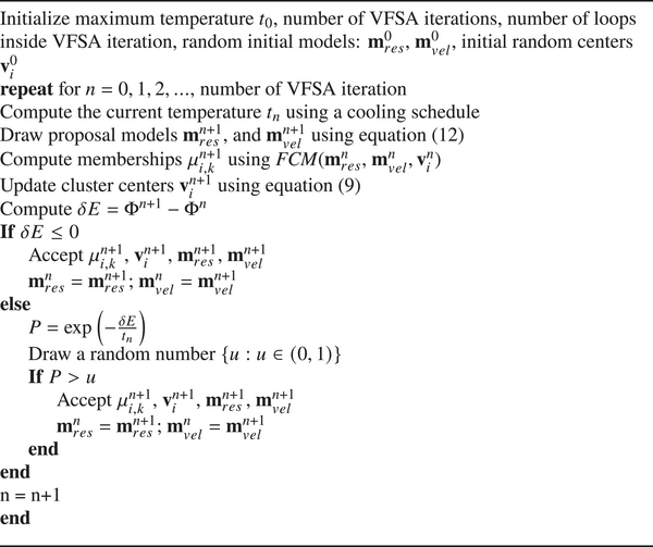
We have normalized individual cost functions for CSEM and seismic with their respective target misfit and do not use relative weights.
3 Test Case
We apply the proposed joint inversion workflow for controlled source electromagnetic (CSEM) and seismic traveltime data generated on a subset of the SEAM Phase I model (Pangman 2007). The SEAM Phase I model is a widely used benchmark in geophysical exploration research that simulates realistic subsurface conditions, including salt structures, for validating inversion methods. The subsurface model built on the SEAM Phase I dataset mimics a realistic geology of a salt-containing region in the Gulf of Mexico (Fehler and Keliher 2011). There is a massive salt body with steep flanks embedded into a layered sediment environment. The velocity model has complex geometrical structures and strong velocity variations that make seismic imaging below salt: challenging. The top boundary of the salt is rugose and has a thin layer of muddy salt having a velocity slightly lower than the main salt body. Since we use using only first-arrival traveltime data for this numerical test, we restrict our area of interest to depth. The SEAM model for this test is a subset of a 2D slice of the original 3D model (at north = ) having a dimension of . The model has a seawater layer of vertical resistivity and P-wave velocity, and the thickness of the seabed varies from to . The true synthetic models for this experiment are shown in Figure 2. The sediments on either side of the salt body have some interesting formations, which are not visible in the velocity model but are prominent in the vertical resistivity model. A preliminary cluster analysis of this cross-plot between true model parameters shows that the geology of the model can reasonably be described with five clusters. We will assume these cluster centres as a prior geological information about the facies in the model. The goal of this numerical test is to perform the joint inversion of seismic and CSEM data over this SEAM model using the given petrophysical and geological constraints and quantify the uncertainty in the estimated models.

For the seismic data, we assumed a typical ocean bottom seismometers profile with 34 receivers uniformly distributed every , with the seismic wavefield downward extrapolated to the seafloor (Arnulf et al. 2011, 2014). For the seismic modelling, we took advantage of the source–receiver reciprocity. As such, we are modelling 34 shots, uniformly distributed at the ocean bottom between to and receivers at a interval. For CSEM modelling, we have used 17 sources between and and receivers at every . The CSEM source is an oriented horizontal electric dipole, which is towed above the seabed, and receivers are at seabed depth. We use two frequencies and and set their corresponding maximum offset to and , respectively. Forward modelling for both methods has been done on regular grids (); however, for the inversion, we use a sparse parameterization approach. That is, we interpolate models on 400 randomly generated points for very fast simulated annealing (VFSA) inversion. Once a model is accepted, we transform the model back to an orthogonal grid for forward computations. The interpolation of the model on the sparse grid uses a linear radial basis interpolation. The choice of the number of points for the sparse parameters is a trade-off between how well it can capture the features of the model and how long it takes for the VFSA algorithm to converge.
Since the water layer is known as a prior, we perturb models only below that. For sparse parameterization, we fix 400 inversion points (same for both models) for one chain and do scattered data interpolation to transform the perturbation to regular modelling grids.
For each VFSA chain, the sparse parameterization was randomly generated (see the Supporting Information). As such, each starting model sampled a different spatial location of the model space. For this experiment, we have run 15 different chains (the initial models and inversion points are shown in the Supporting Information). For fuzzy c-means (FCM) parameters, we assume four clusters (not including the water layer) in the model and provide prior centres (with prior weight ) as deduced from the true models. For a real dataset, these centres would be inferred using the prior knowledge about the subsurface. Figure 3 shows the resistivity and velocity model recovered in one-chain of the joint inversion. The probabilistic nature of the joint inversion workflow allows us to generate a number of models, which can be used to compute uncertainty in the model via statistical analysis. We compute mean, median and uncertainty in the joint inversion for 15 independent chains of VFSA for 3000 iterations. Since a single chain of VFSA provides one model (unlike sampling methods), the mean is calculated from the final models of each chain. Figure 4a,b shows the mean and median resistivity models. The top of the main salt diaper and the flanks are recovered. The reservoir is also clearly visible; however, and the left flank of the salt are not clearly resolved. Similarly, the reservoirs on the right side of the salt and are recovered together and not clearly distinguished. The background sediments are well-recovered. Due to the lack of EM signal in the bottom corners as well as inside the salt body, we see higher uncertainties in those areas as shown in Figure 4c,d. We notice that the reservoirs in the inverted models are slightly deeper than their location in the true resistivity model. As far as the velocity model is concerned, the top boundary of the salt is well resolved. The salt boundary is clearly visible as shown in the mean and median models in Figure 4e and 4f, respectively. The background sediments are well recovered except for the bottom corners and lower part of the salt, which is due to the lack of rays passing through these areas. Given that we started with random initial models, the estimated models from the joint inversion show excellent agreement with the true synthetic models.


The joint inversion framework allows us to manually decide the weight of the prior cluster centres by adjusting the value of the parameter . A smaller value of shows less prior constraints and final cluster centres are mostly recovered through the inversion. A higher value of , on the other hand, does not let the centres in the proposal model move too far away from the prior centre by forcing a high prior constraint. For example, Figure 5a shows the cross-plot between velocity and resistivity of the true synthetic model clustered by using FCM with five centres. Using these centres as priors, Figure 5b,c shows the recovered petrophysics from the joint inversion with and .

Figure 6 shows the posterior probability density of five vertical profiles in both the estimated resistivity (top row) and the estimated P-wave velocity model (bottom row). Assuming the estimated values at each location (not the estimated models themselves) in all the chains have the Gaussian distribution, the posterior probability distribution (PPD) has been computed using histograms. In the resistivity models, the profile at passes through the reservoir between depth. The uncertainty at the top of is less than that of the bottom of , which means that the upper part of is better resolved than the lower part. The vertical profile at passes through a part of the reservoir between depth. Since is close to the salt diapir, it is not as well resolved as . The vertical profile at passes through the salt diapir between depth. This profile shows that the uncertainties are lower near the boundary of the salt and higher as the observation point goes towards the centre of the salt. The uncertainty between ( depth) and ( depth) in the vertical profile at have lower uncertainty bounds; however, uncertainties inside the reservoir are relatively higher.

Figure 7 shows the convergence of individual (CSEM and seismic) as well as a total (joint) cost function for 3000 iterations of 15 different chains of VFSA. The individual costs of CSEM and seismic are normalized by their target errors, that is, 1 and 0.01, respectively. The convergence plots show that the joint inversion converges in 3000 iterations of VFSA and uses approximately equal weight of individual cost functions. This shows that VFSA is a more affordable alternative to Monte Carlo or Markov Chain Monte-Carlo methods, which require thousands of iterations to reach convergence for posterior analysis.

4 Conclusions
We have proposed a probabilistic workflow for joint inversion and uncertainty estimation, incorporating petrophysical and geological constraints. We applied this workflow to the joint inversion of controlled source electromagnetic and seismic synthetic data from the SEAM Phase I model. The workflow efficiently integrates petrophysical constraints and prior geological knowledge of the model. With better priors, such as facies interpreted from existing well logs, one can assign a significantly higher prior weight, causing the joint inversion to more rigorously honour the geological information.
We have demonstrated that VFSA with sparse parameterization converges faster and enables the affordable computation of multiple chains, which in turn provides uncertainty estimates in the model. The generalized fuzzy c-means approach can accommodate different distance measures, which are necessary for efficient clustering based on the statistical relationships between model parameters. VFSA achieves a balance between the efficiency of deterministic methods and the robustness of sampling-based approaches. However, its performance depends on the chosen cooling schedule and, for certain configurations, it can become trapped in local minima. It should also be noted that the required number of iterations, although significantly fewer than those needed for Markov chain Monte Carlo methods, are still substantially higher than those typically used in deterministic approaches. For three-dimensional inversion, a more practical application of this stochastic joint inversion approach would be to estimate starting models for deterministic inversion methods given the high computational cost of the forward solvers.
Acknowledgements
The research was funded by TOTAL E and P, Houston, USA. The first author was partially supported by the Research Council of Finland (359261)
Open access publishing facilitated by Geologian tutkimuskeskus, as part of the Wiley - FinELib agreement.