Bayesian Seismic–Petrophysical Inversion for Rock and Fluid Properties and Pore Aspect Ratio in Carbonate Reservoirs
ABSTRACT
Seismic characterization of carbonate reservoirs is a challenging task due to the complex structure of carbonate rocks, where the seismic response is affected by multiple factors such as pore volume and shape as well as changes in mineralogy due to dolomitization and silicification. Hence, the prediction of petrophysical properties from seismic data is often uncertain. For this reason, we propose a statistical inversion method for the estimation of rock properties, where we combine Bayesian inverse theory with geophysical modelling. The geophysical model aims to compute the seismic response based on the rock and fluid properties and pore structure of the carbonate rocks, and it includes rock physics and the amplitude variation with offset models for the seismic response. The Bayesian formulation allows for the solution of the associated inverse problem by computing the posterior distribution of rock and fluid properties and pore structure of the rocks conditioned by the measured geophysical data. The novelty of the proposed method is that the rock physics model can be any petroelastic relation, without requiring any linearization. For the application to the carbonate reservoir, we adopt the self-consistent inclusion model with ellipsoidal pore shapes and Gassmann's equation for the fluid effect; however, the inversion can be applied to any rock physics model. The statistical model assumes that the prior probability distribution of the model variables is a Gaussian mixture model such that distinct petrophysical characteristics can be associated with geological or seismic facies. The result of the proposed inversion is the most likely reservoir model of rock and fluid and pore geometry parameters, for example, porosity, pore aspect ratio, and water saturation and the uncertainty of the model predictions. The method is demonstrated and validated on synthetic and real examples using well logs and two-dimensional seismic sections from a pre-salt dataset in Brazil.
1 Introduction
The main objective of static reservoir characterization is the quantitative estimation of petrophysical properties for fluid flow simulation and forecasting of reservoir production. At the reservoir scale, petrophysical properties are generally estimated from seismic data. The inversion process requires the knowledge of a geophysical model as well as the application of mathematical methods to predict the unknown variable from the measured data. Geophysical models allow calculating elastic properties such as P- and S-wave velocity and density and their seismic response from petrophysical properties. In particular, rock physics models provide petroelastic relationships that map petrophysical properties to elastic parameters (Mavko et al. 2009; Grana et al. 2021), and the seismic amplitude variation with offset (AVO) model maps elastic properties to their seismic response (Aki and Richards 2002). These relations are combined with geophysical inverse methods to predict the petrophysical properties of interest from measured seismic data.
Seismic and petrophysical inversion methods are well-established techniques that aim to find the most likely model of rock properties based on its seismic response (Avseth et al. 2005; Latimer et al. 2000). The solution of the seismic inverse problem is generally not unique due to the noise in seismic data and the non-bijectivity of the geophysical models (Tarantola 2013). For this reason, statistical methods are generally recommended to estimate the probability distribution of unknown properties and quantify uncertainty prediction in the most likely models. Statistical methods have been proposed in several applications of seismic inversion, petrophysical characterization and facies classification. Buland and Omre (2003) propose a Bayesian formulation for seismic AVO inversion to estimate the posterior distribution of seismic velocities and density. Avseth et al. (2005) present a Bayesian approach for seismic facies classification. Grana and Rossa (2010) define the Bayesian formulation for petrophysical inversion, and Grana, Fjeldstad, et al. (2017) extend the Bayesian formulation to the joint estimation of petrophysical properties and facies classification by integrating a Markov chain model. The use of statistical methods for petrophysical inversion and facies classification is, often referred to as statistical rock physics (Avseth et al. 2005), to identify statistical approaches for rock physics modelling used to generate multiple petroelastic scenarios consistent with the seismic data and its attributes. A detailed review of the integration of rock physics models in seismic inversion workflows for reservoir characterization studies is presented by Bosch et al. (2010) and Grana et al. (2021).
The application of seismic reservoir characterization methods to carbonate rocks is still challenging due to depositional and/or diagenetic heterogeneities controlling velocity variations (Eberli et al. 2003; Vasquez et al. 2019). The seismic response of fluid-saturated porous carbonate rocks is often difficult to interpret because multiple petrophysical factors, such as pore shape and changes in mineralogy due to dolomitization and silicification, affect reservoir properties. In order to apply seismic and petrophysical inversion methods to carbonate reservoirs, it is necessary to define a rock physics model to link the petrophysical properties to the elastic response. The most natural choice for this task is represented by inclusion models (Mavko et al. 2009). Inclusion models assume that a porous medium can be modelled as a solid phase with a set of porous inclusions modelled according to idealized geometrical shapes, such as spheres, needles, discs and the effective elastic moduli depend on the type of inclusion. In the physical-mathematical formulation of these models, the idealized geometrical shape is parameterized by a single parameter, namely the aspect ratio, which is defined as the ratio of the minor and major axes of the ellipsoids used to geometrically represent the shape of the pores (Berryman 1995; Xu and Payne 2009; Mavko et al. 2009).
Rock physics models provide a powerful means to describe the complex geometry of porous rocks, particularly in carbonate reservoirs, where heterogeneity in pore structure significantly influences petrophysical and geophysical properties (Budiansky 1965; Mori and Tanaka 1973; Kuster and Toksöz 1974; Berryman 1980,1981; Xu and Payne 2009; Mavko et al. 2009). Unlike clastic rocks, which often exhibit relatively uniform pore systems, carbonate formations contain a diverse range of pore types, including interparticle, vuggy, moldic and fracture porosity, each contributing differently to the overall elastic and flow properties of the rock. To accurately represent these complexities, rock physics models incorporate key parameters such as porosity, pore aspect ratio, coordination number and pore connectivity. The aspect ratio, which quantifies the shape of idealized pore geometries, is particularly valuable in capturing the influence of elongated cracks versus more spherical pores on both elastic and transport properties (Xu and Payne 2009). Quantifying aspect ratios and other pore-related parameters are crucial for reservoir characterization, as they directly impact fluid flow and permeability. For instance, elongated or crack-like pores tend to enhance permeability anisotropy, allowing preferential flow paths (Mavko et al. 2009). By estimating these parameters using well-log data, laboratory measurements or inversion techniques, reservoir engineers can better predict fluid movement and enhance reservoir management strategies. Additionally, rock physics models linking pore geometry to permeability provide insights into recovery efficiency, helping optimize production in carbonate reservoirs. These pore-scale parameters also play a critical role in controlling seismic responses. The aspect ratio of pores affects the effective elastic moduli, influencing seismic wave velocities and attenuation. Low-aspect-ratio pores, such as cracks and fractures, significantly reduce P-wave and S-wave velocities due to their strong compliance, leading to pronounced anisotropy in seismic data. Furthermore, fluid-filled pores alter seismic signatures through dispersion and attenuation mechanisms, particularly in partially saturated conditions (Mavko et al. 2009). Understanding these relationships enables improved seismic interpretation, enhancing the reliability of direct hydrocarbon indicators and reservoir characterization efforts.
This work focuses on the estimation of porosity, pore aspect ratio and fluid saturation from seismic data. Methods focusing on the estimation of the aspect ratio have been proposed in the literature. Zhao et al. (2013) and Teillet et al. (2021) propose inversion methods to estimate pore types and quantify their effects on carbonates using porosity and elastic logs. Q. Guo et al. (2021) use an empirical relation between the aspect ratio and the petrophysical properties in sandstones. Q. Guo et al. (2022) propose a Monte Carlo-based joint inversion for estimating porosity, fluid saturation and pore aspect ratio. Wang et al. (2023) and Q. G. Guo et al. (2023) use a linearized rock physics parameters model in a joint inversion for the estimation of elastic moduli, density and the pore structure parameters. However, the estimation of the porosity, pore aspect ratio and fluid saturation in a statistical formulation often requires the linearization of the rock physics model. Q. G. Guo et al. (2023) show that the linearization can be derived using Taylor's first-order approximation of the rock physics model; but, the linearization might fail for some of the values close to the boundaries of the physical domain of the petrophysical properties. To overcome this challenge, we present a Bayesian inversion approach where the main novelty is the use of the full rock physics model without any linearization of the equation. In addition, we present a statistical model based on Gaussian mixture models where the components of the mixture distribution can be associated with the carbonate facies of the reservoir. Finally, the uncertainty is fully propagated from the seismic to the petrophysical domain using a hierarchical approach.
The proposed Bayesian inversion method aims to estimate petrophysical and pore geometry parameters (porosity, fluid saturation and aspect ratio) from AVO seismic data. The geophysical model combines the self-consistent inclusion model (Berryman 1995), Gassmann's equation and the Aki–Richards approximation to map rock properties into seismic response; however, the inversion method can be applied to any inclusion model where the pore shape is modelled by a geometrical parameter. We formulate the inverse problem in a statistical framework where the joint probability distribution is assumed to be a Gaussian mixture due to the multi-modality of the rock properties and the non-linearity of the rock physics model. This approach is tested on one-dimensional synthetic data as well as on a set of well logs and a two-dimensional seismic section from a pre-salt dataset in Brazil. The results of the inversion include the most likely model of petrophysical and pore geometry parameters and the uncertainty of the model predictions. We discuss and validate the geological interpretation of the results based on the results of laboratory analysis.
2 Methodology
In this section, we present the Bayesian inversion method proposed for the estimation of petrophysical properties. We first present the geophysical model, including the rock physics and the seismic AVO equation. Unlike previous works (Q. G. Guo et al. 2023), the rock physics model is not linearized and the original formulation is adopted in the inversion. We then present the Bayesian inversion method that is based on a two-step approach: first the seismic inversion is performed, and then the petrophysical inversion is applied. Because each inversion step is formulated in a Bayesian setting, the result of each step is a statistical model. For Bayesian seismic and petrophysical inversions, we combine the two probability distributions: the probability of elastic properties from seismic amplitude variation with offset (AVO) inversion and the probability of petrophysical properties from rock physics inversion, to obtain the posterior distribution of petrophysical properties conditioned on seismic data. We refer to this inversion method as Bayesian seismic–petrophysical inversion. This approach is compared to the Bayesian petrophysical inversion, where the inversion is applied to elastic attributes instead of seismic data, hence ignoring the uncertainty in the prediction of elastic attributes from seismic data.
2.1 Rock Physics Model
A rock physics model is a set of equations that provides a link between elastic properties and petrophysical variables. The model selection depends on the rock type and the geology of the area under study (Mavko et al. 2009; Grana et al. 2021). In this work, for applications to carbonate reservoirs, we use Berryman's self-consistent inclusion model (Berryman 1995) in the formulation described in the following.
2.2 Seismic Amplitude Variation With Offset Model
This formulation can be combined with the rock physics model to predict the seismic response of a sequence of layers with known petrophysical properties, such as porosity, aspect ratio and fluid saturation.
2.3 Bayesian Inversion
2.3.1 Bayesian Seismic Inversion
We adopt the formulation presented in Buland and Omre (2003). We assume that the model variable consists of the logarithm of elastic properties, , and follows a multivariate Gaussian distribution, , with prior mean and spatially correlated prior covariance matrix . This matrix is given by the Kronecker product of the stationary covariance of the model and the spatial correlation matrix defined by a prior spatial correlation function , that is, . Due to the linear approximation of the seismic AVO model in Equation (15), the seismic data vector in Equation (16) is also distributed according to a Gaussian distribution with mean and covariance matrix , where is the first derivative of the mean and is the second derivative of the covariance matrix. We assume that the error is distributed according to a Gaussian distribution with 0 mean and covariance matrix .
2.3.2 Bayesian Petrophysical Inversion
2.3.3 Bayesian Seismic–Petrophysical Inversion
The joint seismic and petrophysical inversion methods can be implemented according to two different strategies. In the simplified two-step approach, we calculate the distribution of elastic parameters from the Bayesian seismic AVO inversion, but the petrophysical parameters are calculated only from the expected values of and do not account for their uncertainty. In the Bayesian seismic–petrophysical inversion, the uncertainty of elastic attributes must be propagated in the petrophysical domain using an integral form for the calculation of the posterior conditional probability as shown by Grana et al. (2021).
In our implementation, the two probabilities in the integral are evaluated for a finite set of combinations of elastic properties and then stored in matrices. The probability is stored in a matrix where each row corresponds to a set of petrophysical property values, and each column corresponds to a set of elastic property values. The probability is stored in a matrix where each row corresponds to a set of elastic property values, and each column corresponds to a seismic trace. The integral is then efficiently computed as a matrix multiplication. The result of an integral is the posterior distribution of petrophysical properties , which is not Gaussian. Hence, the statistical estimators such as mean and variance must be assessed numerically. For the implementation details, we refer to Grana et al. (2021). This approach can also be extended to non-Gaussian distributions as shown by Grana (2022).
3 Application
In this section, we present three applications. In the first and second applications, we generate a set of synthetic well logs using geostatistical simulations and invert the corresponding synthetic seismic trace to validate the inversion method. In the first case, the petrophysical properties show a distinct signature in each facies, whereas in the second case we use real data to generate a synthetic example with overlaps of petrophysical properties within facies. In the third application, we apply the proposed method to a real dataset, including well log and seismic data. The real data are from a carbonate reservoir with partial oil saturation in a pre-salt region of the Santos basin, offshore Brazil. We first apply the inversion to the seismic traces measured at the locations of two wells and then to the two-dimensional (2D) seismic section.
3.1 Synthetic Case 1
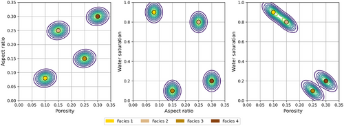
To test the methodology, we created a one-dimensional (1D) synthetic dataset with four facies representing different pore geometries with porosity ranging from low to high, multiple levels of partial saturation and pore spaces with different aspect ratios. Facies are defined based on petrophysical properties, namely porosity , aspect ratio and water saturation . We identified the following facies: Facies 1 represents water-saturated low-porosity rocks with ellipsoidal pores; facies 2 represents water-saturated medium-porosity rocks with rounded pores; facies 3 represents oil-saturated medium-porosity rocks with ellipsoidal pores; and facies 4 represents oil-saturated high-porosity rocks with rounded pores. The continuous properties are distributed according to a multivariate Gaussian mixture with four components, as shown in Figure 1. We simulated well logs by sampling values from the Gaussian mixture model using an exponential spatial correlation function (Grana et al. 2021). We also simulated a facies profile using a first-order Markov chain model (Grana, Fjeldstad, et al. 2017) with transition probability matrix , such that and for , where and represent the and facies. We combined these simulations to create geologically realistic well logs. Figure 2a shows a set of simulated well logs with the corresponding simulated facies.
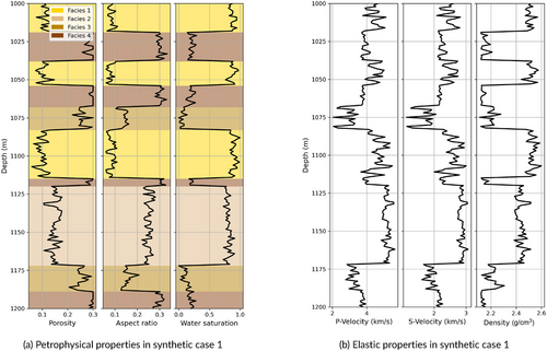
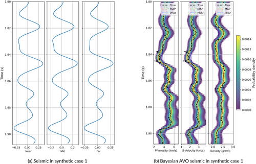
We then apply the rock physics model (Equations 1-12) to calculate elastic properties from the simulated logs as shown in Figure 2b. We assume the following rock and fluid parameters: ; ; and fluid parameters ; ; ; . The seismic data are calculated with the convolutional model in Equation (15) for three angle stacks (near, mid and far, corresponding to 15, 30 and 45 degrees) using a Ricker wavelet with a dominant frequency of 45 Hz for all angle stacks (Figure 3b).
For the inversion, we assume that porosity varies between 0 and 0.4, the aspect ratio between 0 and 0.99, and water saturation between 0 and 1. The true petrophysical properties are not used in the inversion, whereas the true elastic properties are only used for the estimation of the low-frequency model. We first apply the Bayesian petrophysical inversion to the elastic well logs in order to investigate the ability of the inversion to predict the petrophysical properties of interest from high-resolution data without accounting for the uncertainty associated with seismic inversion results. The joint Gaussian mixture model is calibrated using the expectation–maximization algorithm (Grana and Rossa 2010), assuming four components in the domain of the normalized variables. The inversion is performed in a depth domain, and the results in Figure 4a show a high accuracy of the predictions as well as low uncertainty.
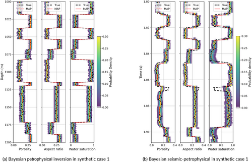
Then, we extend the inversion to the seismic data in order to account for the uncertainty due to the limited seismic bandwidth. We apply the Bayesian seismic amplitude variation with offset (AVO) inversion to the set of seismograms to estimate the posterior distribution of P- and S-wave velocities and density. The low-frequency model is obtained by filtering the log data using a low-pass filter. In inversion, we assume a noise model with zero mean and variance . The results are shown in Figure 3b and are relatively accurate, but they reflect the lower resolution of the seismic data with respect to the well log data. Finally, we apply the proposed Bayesian seismic–petrophysical inversion. The inversion is performed in the time domain. Figure 4b shows the results of the inversion, including the posterior probability distribution of porosity, aspect ratio and water saturation obtained from the petrophysical inversion with seismic uncertainty. The maximum a posteriori model of the posterior probability distributions matches the reference model. The inversion results still show satisfactory accuracy despite some mismatches for layers below the seismic resolution.
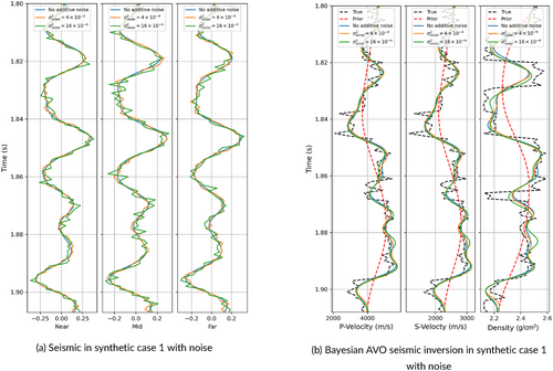
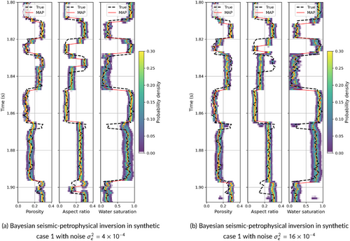
We then test the inversion method assuming two different noise conditions by adding uncorrelated random noise () to the synthetic seismograms. The first example includes an optimistic noise model generated from a Gaussian distribution with zero mean and variance corresponding to a signal-to-noise ratio of approximately 40, whereas the second example includes a more realistic noise model generated from a Gaussian distribution with zero mean and variance , corresponding to a signal-to-noise ratio of approximately 10. Figure 5a shows the seismic traces with and without noise, and Figure 5b shows the predicted values of the elastic properties. Overall, the Bayesian seismic AVO inversion shows consistent results for noisy data. Figure 6a,b shows the results of the Bayesian seismic–petrophysical inversion for the two noise models. In general, the results are consistent with the results in Figure 4b despite a few mismatches at the thin layer boundaries.
| Porosity | Aspect ratio | Water saturation | |
|---|---|---|---|
| Root mean squared errors | |||
| Petrophysical inversion | 0.0131 | 0.0144 | 0.0406 |
| seismic–petrophysical inversion | 0.0340 | 0.0363 | 0.1423 |
| Seis-petro inversion | 0.0371 | 0.0600 | 0.1434 |
| Seis-petro inversion | 0.0422 | 0.0724 | 0.1745 |
| Relative root mean squared errors (%) | |||
| Petrophysical inversion | 0.45 | 0.48 | 0.43 |
| Seismic–petrophysical inversion | 1.63 | 1.65 | 2.03 |
| Seis-petro inversion | 1.78 | 2.73 | 2.04 |
| Seis-petro inversion | 2.02 | 3.29 | 2.48 |
| 0.9 coverage ratio | |||
| Petrophysical inversion | 0.9303 | 0.8756 | 0.8706 |
| Seismic–petrophysical inversion | 0.7248 | 0.7706 | 0.7615 |
| Seis-petro inversion | 0.6881 | 0.6972 | 0.7615 |
| Seis-petro inversion | 0.6147 | 0.6330 | 0.7339 |
Figure 7 shows the comparison between the modelled and predicted MAP for the two inversion approaches. The coefficients of determination () are 0.987, 0.989 and 0.993 for porosity, aspect ratio and water saturation, respectively, for petrophysical inversion (red symbols); 0.908, 0.919 and 0.913 for the seismic–petrophysical inversion without noise (green symbols); 0.886, 0.776 and 0.909 for the seismic–petrophysical inversion with noise (blue symbols); and 0.850, 0.666 and 0.864 for the seismic–petrophysical inversion with noise (cyan symbols).

3.2 Synthetic Case 2
To validate the methodology in a more realistic case with an overlap of petrophysical properties between facies, we created a second 1D synthetic dataset. We used five facies, with statistical parameters of petrophysical properties estimated from a set of real well log data from a borehole located in a carbonate reservoir with partial oil saturation in a pre-salt region of the Santos basin, offshore Brazil. Based on geological stratigraphy and core sample analysis, we identify five petrophysical facies: facies 1, high-porosity carbonate with ellipsoidal pores; facies 2, water-saturated low-porosity carbonate; facies 3, mid-porosity carbonate with ellipsoidal pores; facies 4, mid-porosity carbonate with rounded pores; and facies 5, high-porosity carbonate with rounded pores.
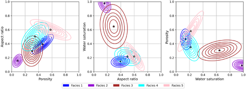
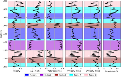
The joint probability density function in the combined petrophysical and elastic domain estimated assuming a Gaussian mixture model with five components using the expectation–maximization algorithm (Grana and Rossa 2010) is shown in Figure 8. The data have been normalized for the application of the expectation–maximization algorithm. For simplicity, we show marginal distributions in the petrophysical domain. The stars represent the mean of the components, and the coloured lines represent the contours of the probability distributions. This statistical model represents a more realistic distribution compared to the previous example. As in the previous example, we use the Gaussian mixture model to generate a set of synthetic well log data. The new synthetic dataset is shown in Figure 9. We assume a statistical model for the error term represented by a Gaussian distribution with zero mean and variance .
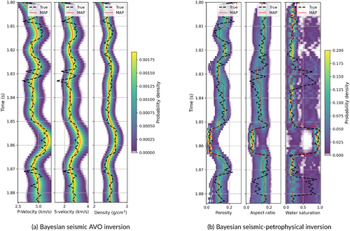
We then apply the proposed method to obtain the posterior probability distributions for the elastic and petrophysical properties. Figure 10 shows the results of the Bayesian seismic AVO inversion and the Bayesian seismic–petrophysical inversion. The results show a satisfactory estimation of the petrophysical variables with smaller uncertainty in the homogeneous layers and larger uncertainties in the layers with a large overlap of properties between facies. The prediction of water saturation shows some mismatches possibly due to the lack of data for the calibration of the joint distribution in the fully water-saturated regions. The RMSE and RRMSE between the measured data and the inversion predictions are shown in Table 2.
| Porosity | Aspect ratio | Water saturation | |
|---|---|---|---|
| Root mean squared errors | |||
| Synthetic from well data | 0.0339 | 0.0346 | 0.2461 |
| Relative root mean squared errors (%) | |||
| Synthetic from well data | 2.78 | 2.83 | 5.56 |
| 0.9 coverage ratio | |||
| Synthetic from well data | 0.7882 | 0.8235 | 0.9294 |
3.3 Real Case Application
The real dataset is from an oil-saturated carbonate reservoir in a pre-salt region of the Santos basin, offshore Brazil. The Santos Basin is a sedimentary basin that contains oil and gas reserves beneath a 2000-meter-thick layer of salt. The pre-salt region is 120 miles wide and runs 500 miles along the coast, and it is one of the most prolific deep-water oil regions in the world, with reservoirs ranging from 18,000 to 25,000 ft below sea level. The stratigraphy of the Santos basin can be divided into three main zones: (i) rift, with basaltic outflows and siliciclastic, coquinas and shale deposits in the Camboriú, Piçarras and Itapema formations; (ii) post-rift, with microbial lacustrine carbonates and evaporites in the Barra Velha and Ariri formations; and (iii) drift, with siliciclastic deposits (Lima and De Ros 2019; Silva Adriano et al. 2022; Chinelatto et al. 2020). The carbonate reservoirs are associated with lacustrine systems in the Itapema and Barra Velha formations, and these rocks are known for their complexity, due to the high variability of depositional facies and diagenetic processes (Rebelo et al. 2023). The overlying salt layer in the Ariri formation is made up of halite, anhydrite, and other evaporites, which create reservoir traps for the hydrocarbons below it. In this dataset, two boreholes are available, namely well A and well B. Seismic data was acquired with ocean bottom node technology and processed using least-square reverse time migration. The interval under consideration in this study is partially saturated with oil. The oil–water contact can be accurately detected in the borehole locations, at 5785 m. The saturation parameters are estimated from the fluids sampled at the well locations.
3.3.1 Well Log Data
Well logs of petrophysical and elastic properties, including porosity, water saturation, P- and S-wave velocity and density, are available at two borehole locations. We use data from well A as training data to define the Gaussian mixture model and data from well B as testing data to assess the inversion results. Within the reservoir interval, saturation does not show significant variations and irreducible water saturation varies between 0.1 and 0.2. The mineralogy of the reservoir is similar in all zones; however, due to differences in depositional evolution and diagenetics, different pore structures are expected in these zones, leading to different elastic and petrophysical properties. Because direct borehole measurements of the aspect ratio are not available, we compute a profile of values of effective pore aspect ratio that optimize the rock physics predictions for elastic properties at each depth. This computed profile is only shown as a reference profile, and it is not used in the inversion. The rock physics model is calibrated at the well location to match the porosity, density, and sonic log measurements. The matrix parameters are ; ; and the reservoir fluids are brine and oil, with parameters ; ; ; .
Figures 11 and 12 show the petrophysical and elastic logs (black lines) and the predictions of the rock physics model (red lines) in the two wells. The magenta dashed lines show the geological markers that delimit stratigraphic zones. This classification is provided for visualization purposes, but is not used in the inversion. Zones 1 and 2 are part of the Barra Velha formation, while zone 3 is classified as Itapema. According to the given zone classification, we observe slightly higher aspect ratio values in zone 2, despite similar porosity values compared to the other zones.
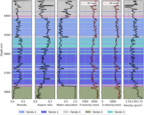
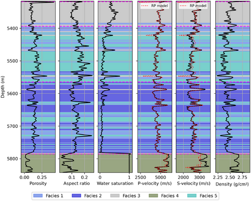
We define a facies classification that includes five facies: facies 1, mid-porosity carbonate with rounded pores; facies 2, mid-porosity carbonate with ellipsoidal pores; facies 3, low-porosity carbonate with ellipsoidal pores; facies 4, water-saturated low-porosity carbonate; and facies 5, high-porosity carbonate with rounded pores. The number of components in the Gaussian mixture model is considered a hyperparameter of the inversion. Using a limited number of components might result in an overestimation of the uncertainty, and the predictions might tend to regress to the mean components. Instead, using a large number of components might result in an underestimation of the uncertainty since it is equivalent to restricting the model space by introducing additional constraints. Generally speaking, the number of components should be related to the number of seismically recognizable geological facies. For this reason, we suggest adopting a number between 3 and 6. The Gaussian mixture model estimated in well A and the well log data from well A are shown in Figure 13.

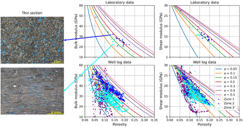
We validate the rock physics model using core sample measurements. Figure 14 shows rock physics templates, together with laboratory and well log measurements, and thin sections from two core samples, to illustrate the difference in the elastic behaviour of rocks in different stratigraphic zones. The plot indicates that changes in the aspect ratio allow for discriminating different elastic behaviours according to the pore geometries in the thin sections, where we observe more rounded pores in zone 2 and more elongated pores in zone 3. In fact, coquinas in the Itapema formation typically consist of rudstones and grainstones from bivalve and gastropod shells (Chinelatto et al. 2020), resulting in more elongated pore geometries, while the rocks of the Barra Velha formation are mostly made of laminated carbonates, magnesian clay minerals, calcite spherulites and shrubs (Rebelo et al. 2023; Gomes et al. 2020), resulting in more rounded pores.
We then apply the proposed method to seismic traces measured at the borehole locations. The low-frequency model for the Bayesian seismic AVO inversion is estimated from well log data. The posterior distributions of porosity, aspect ratio and water saturation are shown in Figure 15 for wells A and B. The RMSE and RRMSE between the measured data and the inversion results and the 0.9 coverage ratios of the predictions are shown in Table 3.
| Porosity | Aspect ratio | Water saturation | |
|---|---|---|---|
| Root mean squared errors | |||
| Well A | 0.0336 | 0.0367 | 0.3019 |
| Well B | 0.0423 | 0.0416 | 0.1553 |
| Well A (upscaled) | 0.0311 | 0.0266 | 0.2418 |
| Well B (upscaled) | 0.0236 | 0.0298 | 0.1075 |
| Relative root mean squared errors (%) | |||
| Well A | 1.92 | 1.98 | 4.49 |
| Well B | 1.98 | 1.95 | 2.79 |
| Well A (upscaled) | 1.75 | 1.45 | 3.66 |
| Well B (upscaled) | 1.14 | 1.45 | 1.99 |
| 0.9 coverage ratio | |||
| Well A | 0.7746 | 0.8779 | 0.8826 |
| Well B | 0.7186 | 0.8750 | 0.5491 |
| Well A (upscaled) | 0.8910 | 0.9014 | 0.9108 |
| Well B (upscaled) | 0.8616 | 0.9286 | 0.6250 |
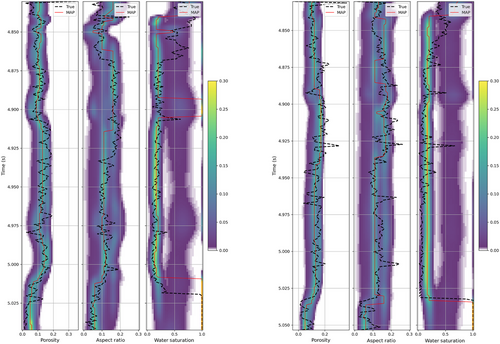
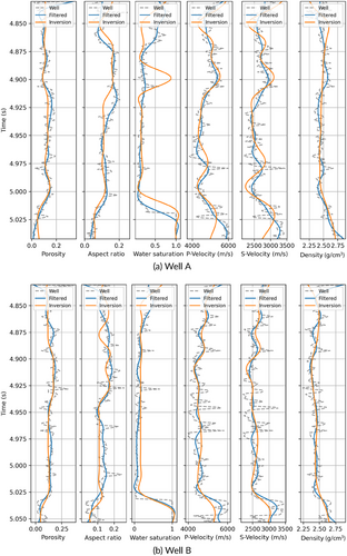
To assess the accuracy of the results obtained by Bayesian seismic–petrophysical inversion, we compare the inverted properties to the well log data in the time domain after upscaling the measured data according to the frequency of the measured seismic data. Elastic logs have been upscaled using the Backus average, whereas petrophysical logs have been upscaled using a moving average. Figure 16 displays the inversion results and the upscaled well logs in the time domain, illustrating a satisfactory agreement between the inverted and upscaled properties. The RMSE and RRMSE between the upscaled well logs and the inversion results and the 0.9 coverage ratios of the predictions are shown in Table 3.
3.3.2 Two-Dimensional Seismic Data
Finally, we apply the proposed method to a 2D section extracted from the three-dimensional (3D) seismic dataset and intersecting the locations of well B. The section contains 140 traces in the time domain. The well log data from well A was used as training data to estimate the joint multivariate Gaussian mixture of petrophysical and elastic properties, assuming five Gaussian components corresponding to the five petrophysical facies identified in the Gaussian mixture distribution, as in the previous example.
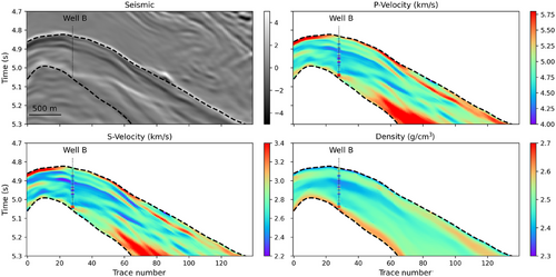
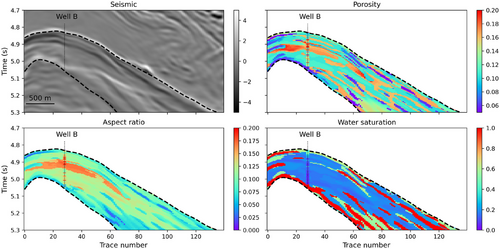
We apply the Bayesian seismic and petrophysical inversion to obtain the posterior distribution of P- and S- wave velocity and density as well as porosity, aspect ratio and water saturation. Figure 17 and Figure 18 shows the inversion results where the well log data from well B are superimposed for comparison. The sections of the MAP values of porosity and water saturation show an accurate match with the upscaled well log data as well as a strong lateral structure. The section of the most likely values of the aspect ratio identifies a layer of higher values corresponding to the top of stratigraphic zone 2, confirming the different elastic behaviour between the stratigraphic zones identified at the well locations (Figure 14). However, water saturation predictions show high values at discontinuous intervals, which is not present in the well data.
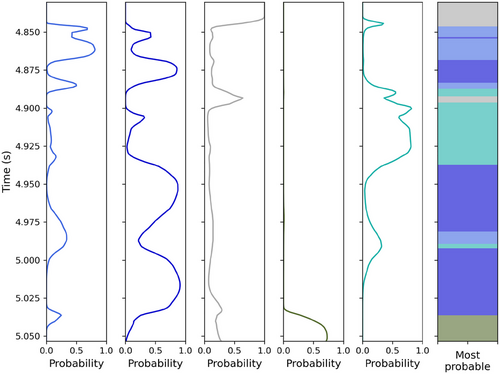
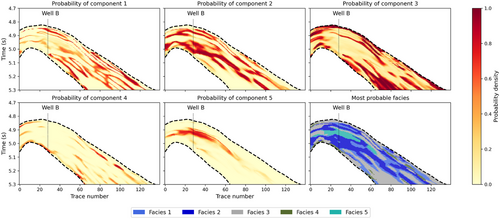
In addition to the posterior distribution of elastic properties, the Bayesian seismic–petrophysical inversion also provides the posterior probability of the Gaussian components, which in our approach are assumed to be equal to the posterior probability of the petrophysical facies (Equation 23). Figure 19 shows the posterior probability of the five petrophysical facies and the most likely facies model in well B. The results are consistent with the facies definition in Figure 12, as well as prior geological information, and the stratigraphic model. Figure 20 shows the predicted probabilities and the most likely model, illustrating a satisfactory correlation with the predicted petrophysical properties.
4 Discussion
The proposed method aims to provide an efficient and accurate solution for the prediction of rock and fluid properties from seismic data in carbonate reservoirs. In this section, we address assumptions, advantages and limitations of the proposed methodology.
4.1 Rock Physics Model Assumptions
Rock physics models based on the concept of inclusions have been developed to analyse the elastic behaviour of heterogeneous formations, and are particularly useful in carbonate reservoirs. The theory of inclusion-based rock physics models relies on the foundational works by Budiansky (1965); Mori and Tanaka (1973); Kuster and Toksöz (1974); Berryman (1980) and Berryman (1981). Budiansky (1965) introduced an initial approach for representing the elastic characteristics of composite materials. Mori and Tanaka (1973) developed a method to estimate the distribution of stress and strain in a matrix containing inclusions. Kuster and Toksöz (1974) later refined this approach to model how seismic waves travel through and attenuate within two-phase systems. Norris (1985) formulated a differential effective medium approach to account for variations in moduli of composite substances. In addition, Berryman (1980) employed long-wavelength approximations to investigate wave movement in materials with spherical inclusions. These theoretical models have been applied to carbonate formations for understanding complex pore structures. For example, Xu and Payne (2009) adopted inclusion-based models to estimate the elastic properties of carbonate reservoirs and investigate the effect of pore shape and connectivity. In these models, inclusions can be modelled in dry or saturated conditions. Any of these rock physics formulations can be integrated into the proposed Bayesian inversion methodology. Because the rock physics model is applied to data measured at seismic frequencies, in our work, we adopted the dry formulation combined with Gassmann's equation, but the inversion could be extended to formulations with saturated inclusions.
4.2 Gaussian Mixture Prior Model
We assume that petrophysical properties are distributed according to a Gaussian distribution within each facies. This assumption is equivalent to assuming that petrophysical properties are distributed according to a Gaussian mixture model, which is defined as a linear combination of Gaussian distributions. The weights of the mixture represent the facies proportions as shown in Grana and Rossa (2010). For the calibration of the Gaussian mixture model, we use the expectation–maximization method, an iterative algorithm for finding the maximum likelihood estimates of a set of statistical parameters (mean and variance, for instance), in datasets where the model depends on an unknown categorical variable (facies, in our case). The algorithm is considered unsupervised, but it requires initial guess values of the parameters. Hence, we can include prior geological information in the initial values to constrain the classification. The iterative approach allows for an adaptive refinement of facies probabilities, improving classification accuracy with each step. The expectation–maximization method provides a powerful probabilistic framework for facies classification by using probabilistic distributions rather than a deterministic classification. The algorithm offers additional flexibility by allowing for the incorporation of different statistical distributions, making it adaptable to diverse geological environments. Grana, Lang, et al. (2017) study the accuracy and efficiency of Gaussian mixture models and expectation–maximization for the facies classification by comparing the results to the standard Bayesian classification and also investigate the effects of the number of input variables as well as the number of facies. A prior sensitivity analysis should be conducted to determine the optimal number of facies. Overall, we recommend adopting a number of facies between 3 and 5 to avoid large overlaps of rock and fluid properties and to reduce the entropy associated with complex classifications. In the proposed formulation, we adopted a Gaussian mixture assumption for the flexibility of the model and the analytical tractability of the formulations. A Gaussian model would also offer a tractable mathematical formulation but could not describe the facies-dependent multimodal behaviour of the properties. On the other hand, a non-parametric distribution would offer a flexible model capable of describing the skewness and multimodality of the properties, but could not provide analytically tractable solutions.
4.3 Uncertainty Propagation and Quantification
Uncertainty propagation in petrophysical characterization using a two-stage Bayesian approach, integrating rock physics and seismic inversion via the Chapman–Kolmogorov equation, provides a rigorous probabilistic framework for quantifying subsurface properties. This methodology accounts for uncertainty at multiple levels: the seismic inversion stage, where elastic properties are inferred from seismic data, and the rock physics stage, where these properties are translated into petrophysical parameters. By employing the Chapman–Kolmogorov equation, the approach effectively marginalizes latent variables, ensuring a consistent transfer of uncertainty from seismic data to petrophysical estimates. This not only captures the variability inherent in geophysical measurements but also enhances the robustness of reservoir characterization by integrating prior geological knowledge and observed data within a coherent probabilistic framework. The result is a more comprehensive quantification of uncertainty, which is crucial for reliable decision-making in reservoir assessment and exploration. However, the extent of uncertainty is strongly dependent on the quality of the input data. High signal-to-noise ratios, dense well control and accurate prior geological constraints reduce uncertainty, leading to more reliable petrophysical predictions. Conversely, poor seismic resolution, sparse well data and uncertain rock physics relationships can significantly amplify uncertainty, making it more challenging to obtain precise reservoir characterizations.
4.4 Advantages and Practical Applications
Seismic petrophysical inversion is a powerful tool for hydrocarbon exploration and production, providing a link between geophysical seismic data and reservoir engineering applications. Seismic petrophysical inversion results are crucial for identifying hydrocarbon-bearing zones by transforming seismic reflection data into petrophysical properties, such as porosity, fluid saturation and lithology. These results provide an improved understanding of subsurface reservoirs, particularly in 3D volumes and two-dimensional (2D) sections as well as at well locations. One of the advantages of seismic petrophysical inversion in carbonate reservoirs is the ability to infer the geometry of pore structures, which directly influences reservoir quality. Using parameters such as pore aspect ratio, we can improve estimates of fluid saturation and permeability. The aspect ratio of the pores affects the velocities of the elastic waves, and by incorporating these effects into the inversion workflows, we can more accurately differentiate between well-connected pore systems in high-quality reservoirs and more isolated, crack-like porosity that may reduce permeability. This knowledge improves predictions of fluid flow, and it helps in assessing the productivity potential of a reservoir more effectively. By integrating seismic inversion results with well-log data, we can refine interpretations and improve the lateral continuity of reservoir models and improve resolution in 2D seismic sections and 3D seismic volumes to obtain a better understanding of subsurface heterogeneity. The ability to characterize lithology and reservoir quality helps in identifying optimal drilling targets, reducing exploration risks and improving hydrocarbon recovery. The method is applied to an oil-saturated reservoir, but it could be extended to any fluid type, in particular gas reservoirs. However, in gas reservoirs, it might be challenging to accurately predict partial saturation, due to the non-linear behaviour of the elastic properties of gas-saturated carbonate rocks and the limited sensitivity of seismic data to fluid effects for gas saturation between 0.1 and 0.9 (Mavko et al. 2009). The inversion method can also be extended to other rock types and mineralogies, and more sophisticated rock physics models can be adapted to link petrophysical and elastic properties.
5 Conclusions
The estimation of petrophysical properties from seismic data is a challenging task in carbonate reservoirs due to the complex pore structures. This work presents a Bayesian seismic–petrophysical inversion based on a rock physics model that assumes inclusions characterized by the pore aspect ratio to represent different pore geometries. We proposed a rock physics inversion approach that combines Berryman's self-consistent inclusion model, Gassmann's equation and the seismic amplitude variation with offset model in a Bayesian approach for the prediction of the posterior probability distribution of the petrophysical properties, including porosity, pore aspect ratio and fluid saturation. Due to the non-linearity of the model, it is not possible to derive an analytical expression for the posterior probability; hence, we propose a strategy that combines Gaussian mixture fitting. The definition of geological facies, if available, identifies the components of the Gaussian mixture models; otherwise, the Gaussian mixture distribution can be automatically fitted in the joint elastic and petrophysical domains using the expectation–maximization algorithm. Applications to synthetic and real data show that the method allows for finding accurate estimates of petrophysical properties at the well locations. The larger errors for saturation are possibly due to the limited variability of the saturation in the training data as well as the low sensitivity of seismic data to partial saturation. The aspect ratio estimated in the inversion is a valuable parameter for reservoir model interpretation, forecasting and development.
Acknowledgements
The authors acknowledge Petrobras and the Department of Geology and Geophysics of the University of Wyoming for support.
The Article Processing Charge for the publication of this research was funded by the Coordenação de Aperfeiçoamento de Pessoal de Nível Superior - Brasil (CAPES) (ROR identifier: 00x0ma614).
APPENDIX: Self-Consistent Approximation for Ellipsoidal Inclusions
Open Research
Data Availability Statement
Data are available upon request.


