Volume 70, Issue 1 pp. 3-18
Original Article
Open Access

Homotopy scattering series for seismic forward modelling with variable density and velocity

Kui Xiang

Corresponding Author

Kui Xiang

Department of Earth Science, University of Bergen, Postboks, Bergen, 7803 5020 Norway

E-mail: [email protected]

Search for more papers by this author
Kjersti Solberg Eikrem

Kjersti Solberg Eikrem

NORCE Norwegian Research Centre AS, Postboks 22 Nygårdstangen, Bergen, 5838 Norway

Search for more papers by this author
Morten Jakobsen

Morten Jakobsen

Department of Earth Science, University of Bergen, Postboks, Bergen, 7803 5020 Norway

NORCE Norwegian Research Centre AS, Postboks 22 Nygårdstangen, Bergen, 5838 Norway

Search for more papers by this author
Geir Nævdal

Geir Nævdal

NORCE Norwegian Research Centre AS, Postboks 22 Nygårdstangen, Bergen, 5838 Norway

Search for more papers by this author
First published: 01 September 2021
Citations: 2

ABSTRACT

We have derived a convergent scattering series solution for the frequency-domain wave equation in acoustic media with variable density and velocity. The convergent scattering series solution is based on the homotopy analysis of a vectorial integral equation of the Lippmann–Schwinger type. By using the Green's function and partial integration, we have derived the vectorial integral equation of the Lippmann–Schwinger type that involves the pressure gradient field as well as the pressure field from the wave equation. The vectorial Lippmann–Schwinger equation can in principle be solved via matrix inversion, but the computational cost of matrix inversion scales like N 3 , where N is the number of grid blocks. The computational cost can be significantly reduced if one solves the vectorial Lippmann–Schwinger equation iteratively. A simple iterative solution is the Born series, but it is only convergent when the scattering potential is sufficiently small. In this study, we have used the so-called homotopy analysis method to derive an iterative solution for the vectorial Lippmann–Schwinger equation which can be made convergent even in strongly scattering media. The computational cost of our convergent scattering series scales as N 2 . Our algorithm, which is based on the homotopy analysis method, involves a convergence control operator that we select using hierarchical matrices. We use a three-layer model and a resampled version of the SEG/EAGE salt model to show the performance of the developed convergent scattering series.

INTRODUCTION

The integral equation method is one of the most valuable methods in seismic forward modelling and inversion (Aki and Richards, 1980; Van Den Berg and Kleinman, 1997; Carcione et al., 2002; Abubakar et al., 2003; Innanen, 2009; Jakobsen, 2012; Jakobsen and Ursin, 2015; Malovichko et al., 2018; Huang et al., 2020). It considers the total wavefield in the actual medium as a superposition of a background wavefield and a scattering wavefield. The background wavefield and the scattering wavefield are found from the integral representations in terms of the Green's function and the actual and virtual source. The virtual source is caused by the contrast between the actual medium and the background medium. If the contrast part is compact enough, the computation will be accelerated. Although the integral equation system matrix is relatively small due to the compact contrast part, it is still a full matrix. If we implement it through matrix inversion, it will cause a relatively high memory demand and computational burden (Jakobsen and Wu, 2018), especially when the model is a large-scale model. This fact leads researchers to use iterative methods based on scattering series solutions instead of direct matrix inversion for solving the integral equation. One of the most well-known series solutions in the geophysical community is the Born series solution (Morse and Feshbach, 1954). However, the conventional Born series is only guaranteed to converge when the contrast or the scattering potential of the model is relatively small (Jakobsen and Ursin, 2015; Osnabrugge et al., 2016). Therefore, a lot of effort has been devoted to solving the divergence problem of the Born series in the presence of strong contrasts. Zhdanov and Fang (1997) have generalized the Born series by using the higher order quasi-linear approximations to ensure the modified series converge to the true solution. Osnabrugge et al. (2016) have modified the Born series to converge for high scattering potentials by introducing a pre-conditioner and an auxiliary parameter to localize the energy of the Green's function. Jakobsen and Wu (2016) have replaced the Born series with a convergent renormalized scattering series by utilizing the leading De Wolf approximation. By using the modified volume integral equation proposed by Bonnet and others (2017), Abhishek et al. (2020) have developed a modified Born series, that is unconditionally convergent, for the forward and inverse scattering problem.

All the methods mentioned above assume that the density is constant. But in fact density plays an important role in the amplitude of the wavefield. If we only consider the velocity in wavefield forward modelling when density varies in reality, the synthetic seismic wavefield will not match the observed wavefield well, which may cause serious artefacts in the full waveform inversion (Virieux and Operto, 2009). Many forward modelling methods, most of them for the ultrasound imaging, have been developed with variable density (Kwon and Jeong, 1998; Lavarello and Oelze, 2009; Mojabi and LoVetri, 2015; Rao et al., 2020). In recent years, some studies about integral equation methods for seismic forward modelling with variable density have been considered in several publications (Yang et al., 2016; Yao et al., 2016; Sun et al., 2017; Jiménez et al., 2018; Luo and Wu, 2018; Farshad and Chauris, 2020). Although these studies have been developed, there is still an important need to develop more accurate and efficient methods for seismic forward modelling with variable density. Therefore, in this study, we present a new integral equation scheme applicable in the case of variable density and velocity.

Unlike other seismic forward modelling methods that include density and velocity, we have derived two coupled integral equations and combined them into a vectorial Lippmann–Schwinger (LS) equation. Because there are already many methods for solving the LS equation (Jakobsen and Ursin, 2015; Jakobsen and Wu, 2016; Eftekhar et al., 2018; Huang et al., 2020; Eikrem et al., 2020), we may use those methods to solve the vectorial LS equation. This is our main motivation to extend the previous methods to the variable velocity and density case. Because of the introduction of the density term, the scattering potential involving two parameters in the vectorial LS equation becomes complicated. It is necessary to further develop a convergent scattering series solution for the vectorial LS equation due to the strong scattering potential. In this study, we use the homotopy analysis method developed by Liao (1997, 2003), and Liao and Tan (2007) to solve the vectorial LS equation. There have been many successful applications of the homotopy techniques in geophysics. Keller and Perozzi (1983) introduced continuation in their methods for fast seismic ray tracing. Hanyga and Pajchel (1995) further explored homotopy methods in complicated models. Allgower and Georg (1990) give an introduction to numerical homotopy methods. Huang and Greenhalgh (2018) used the modern homotopy analysis method (Liao, 2003) to solve anisotropic eikonal equation for traveltime approximations. Jakobsen et al. (2020) have proposed a convergent scattering series solution of the scalar LS equation through the homotopy analysis method. Jakobsen et al. (2020) have compared convergence performance of different scattering series derived from homotopy continuation method and renormalization group. Previously, Jakobsen et al. (2020) have concluded that the scattering series solution is guaranteed to converge in fixed density case by introducing a suitable convergence control operator. In the present study, we modify the homotopy analysis method in Jakobsen et al. (2020) to solve the vectorial LS equation. Due to the strong scattering potential in the vectorial LS equation, the simple convergence control operator given in Jakobsen et al. (2020) cannot ensure that the scattering series converges. So we introduced another convergence control operator developed by Eikrem et al. (2020) based on the matrix low rank approximation (Halko et al., 2011) and the hierarchical matrix (Börm et al., 2003). In Eikrem et al. (2020), they mainly focus on the convergence control operator for the scalar LS equation. In this study, we developed a new convergence control operator for the vectorial LS equation based on Eikrem et al. (2020) by constructing hierarchical matrices for different blocks of the full matrix. In principle, if we choose the parameters related to the convergence control operator properly, the homotopy scattering series will converge.

This paper is structured as follows. First we transform the wave equation for acoustic medium into the vectorial integral equation of the LS type. Then we discuss the reference solution from matrix inversion as well as the conventional Born series solution. Next we give a description of the homotopy analysis method and derive the convergent homotopy series solution. Finally we use numerical examples to demonstrate the performance of the proposed method, compare it with the conventional Born series and give the concluding remarks. The formulation of two-dimensional and three-dimensional acoustic Green's functions and their spatial derivatives are given in Appendices A and B.

THEORY

The vectorial Lippmann–Schwinger equation

The acoustic wave equation for heterogeneous medium in frequency domain can be written as (Červený, 2005)
· 1 ρ ( x ) + ω 2 κ ( x ) p ( x , ω ) = S ( x , ω ) , (1)
where is the spatial gradient operator, ω is the angular frequency, κ ( x ) = ρ ( x ) v 2 ( x ) is the bulk modulus related to the density ρ ( x ) and the velocity v ( x ) , p ( x , ω ) is the pressure wavefield in the acoustic medium and S ( x , ω ) represents the source term, x R n is the spatial position, where n = 2 , 3 denotes the dimensionality of the problem. The wavefield p, the source term S and the following Green's functions are all dependent on the angular frequency ω, but we will in the following suppress this dependency for simplicity.
We define the normalized contrasts in the mass density and bulk modulus fields by
χ ρ ( x ) = ρ 0 ρ ( x ) 1 , χ κ ( x ) = κ 0 κ ( x ) 1 , (2)
where ρ 0 , κ 0 = ρ 0 v 0 2 and v 0 are the density, the bulk modulus and the velocity of a homogeneous background model. By combining (1) and (2), we obtain
1 ρ 0 2 + ω 2 κ 0 p ( x ) = S ( x ) · χ ρ ( x ) ρ 0 + ω 2 χ κ ( x ) κ 0 p ( x ) . (3)
We multiply both sides of (3) by ρ 0 and use κ 0 = ρ 0 v 0 2 to get
2 + k 0 2 p ( x ) = ρ 0 S ( x ) · χ ρ ( x ) + k 0 2 χ κ ( x ) p ( x ) , (4)
where k 0 = ω / v 0 is the wave number in the background medium.
The second term on the right-side of the equation (4) can be considered as secondary source. By using the volume integral (Morse and Feshbach, 1954), we represent the wavefield p ( x ) as
p ( x ) = p ( 0 ) ( x ) + d x g ( 0 ) ( x x ) x · χ ρ ( x ) x + k 0 2 χ κ ( x ) p ( x ) , (5)
where
p ( 0 ) ( x ) = ρ 0 d x g ( 0 ) ( x x ) S ( x ) (6)
is the wavefield in the homogeneous background medium due to the actual source S and g ( 0 ) ( x x ) is the Green's function for the homogeneous background medium that satisfies
2 + k 0 2 g ( 0 ) ( x x ) = δ ( x x ) , (7)
where δ ( x x ) is the Dirac delta function and represents a point source. In this paper, we use the Green's function for the homogeneous acoustic medium (see Appendices A and B) to calculate g ( 0 ) ( x x ) . More details about the Green's function can be found in Arfken and Weber (1999).
The appearance of the divergence operator x on χ ρ ( x ) makes the use of equation (5) complicated. By using the rule of divergence of a product (Arfken and Weber, 1999), we have
d x g ( 0 ) ( x x ) x · χ ρ ( x ) x p ( x ) = d x x · g ( 0 ) ( x x ) χ ρ ( x ) x p ( x ) d x x g ( 0 ) ( x x ) · χ ρ ( x ) x p ( x ) . (8)
The first term on the right-hand side of (8) can be converted into a surface integral through Gauss's theorem, which goes to zero because the Green's function and the fields approaches zero at infinity. By combining (5) and (8) and replacing x with x , we obtain:
p ( x ) = p ( 0 ) ( x ) + k 0 2 d x g ( 0 ) ( x x ) χ κ ( x ) p ( x ) + d x x g ( 0 ) ( x x ) · χ ρ ( x ) x p ( x ) . (9)
In equation (9), there is no spatial derivative on χ ρ ( x ) , which is useful for inversion. However, equation (9) also shows we need the spatial derivative of the pressure field to calculate the pressure field itself, which may be difficult for the forward modelling. To mitigate this problem, we take spatial derivative on both sides of equation (9) and obtain
x p x = x p ( 0 ) x + k 0 2 d x x g ( 0 ) x x χ κ x p x + d x x x g ( 0 ) x x · χ ρ x x p x . (10)
Next we combine (9) and (10) into the vectorial Lippmann–Schwinger equation:
ψ x = ψ ( 0 ) x + d x G ( 0 ) x x V x ψ x , (11)
where ψ ( x ) = ( p ( x ) , x p ( x ) ) T and ψ ( 0 ) ( x ) = ( p ( 0 ) ( x ) , x p ( 0 ) ( x ) ) T is the combined wavefield, a ( n + 1 ) × 1 vector, including the wavefield itself and its spatial derivative, in the actual and background medium, respectively;
V x = χ κ x 0 n T 0 n χ ρ x I n (12)
is a ( n + 1 ) × ( n + 1 ) scattering potential operator including the contrast of bulk modulus and density, where 0 n is an n × 1 zero vector and I n is an n × n identity matrix;
G ( 0 ) x x = k 0 2 g ( 0 ) x x x g ( 0 ) x x T k 0 2 x g ( 0 ) x x x x g ( 0 ) x x (13)
is an ( n + 1 ) × ( n + 1 ) operator including the Green's function and its first- and second-order spatial derivatives. More details about the Green's function and its first- and second-order spatial derivatives are given in Appendices A and B for the two-dimensional and three-dimensional cases, respectively.

Matrix representation of the vectorial LS equation

For the sake of simplicity, next we will present the matrix representation of the vectorial Lippmann–Schwinger (LS) equation in two-dimensional (2D) case. However, it can be extended to three-dimensional (3D) easily. We first divide the model into N grid blocks. At each grid block, the combined wavefield, presented by the combined wavefield at the centroid of that grid block, includes the wavefield p and its spatial derivative p . In 2D case, p has two components p 1 and p 2 ; g has two components g 1 and g 2 and g has four components g 11 , g 12 , g 21 and g 22 . Next we formulate the combined wavefield at all points of the discrete domain and rearrange them into vectors ψ = ( p , p 1 , p 2 ) T , where p = ( p 1 , , p N ) T , p 1 = ( p 1 1 , , p 1 N ) T and p 2 = ( p 2 1 , , p 2 N ) T . Finally we obtain the matrix representation of the vectorial LS equation:
ψ = ψ ( 0 ) + G ( 0 ) V ψ , (14)
where
ψ ( 0 ) = ( p ( 0 ) , p 1 ( 0 ) , p 2 ( 0 ) ) T ; (15)
V = χ κ 0 0 0 χ ρ 0 0 0 χ ρ ; (16)
G ( 0 ) = k 0 2 g ( 0 ) g 1 ( 0 ) g 2 ( 0 ) k 0 2 g 1 ( 0 ) g 11 ( 0 ) g 12 ( 0 ) k 0 2 g 2 ( 0 ) g 21 ( 0 ) g 22 ( 0 ) . (17)
In equation (16), χ κ and χ ρ are both an N × N diagonal matrix and 0 is a N × N zero matrix. In equation (17), all blocks of G ( 0 ) are N × N  matrix.
The wavefield ψ in equation (14) can be solved through matrix inversion:
ψ = ( I G ( 0 ) V ) 1 ψ ( 0 ) , (18)
where I is a 3 N × 3 N identity matrix. However, the computational cost of inverting a huge full matrix I G ( 0 ) V scales like N 3 , which is costly due to the large number of grid blocks in practical applications.

The Born series iteration

As mentioned above, solving equation (18) is costly in the realistic case. In order to solve the problem of high-computational cost, we use iterative methods, instead of matrix inversion, to solve equation (14). One of the most well-known iterative methods is the Born series solution (Morse and Feshbach, 1954):
ψ = ( I + G ( 0 ) V + G ( 0 ) V G ( 0 ) V + ) ψ ( 0 ) . (19)
Equation (19) can be rewritten in iterative form as
ψ k = ψ ( 0 ) + G ( 0 ) V ψ k 1 , k 1 , (20)
where ψ k is an estimate of the total wavefield after k iterations, which is equal to the partial sum of the first k terms in (19). When ψ k ψ k 1 is small, the iterations are stopped, and the computational cost of (20) scales as N 2 . The cost is greatly reduced compared with matrix inversion (18). However, the Born series iteration is only guaranteed to converge when the spectral radius, σ ( G ( 0 ) V ) , is smaller than unity, which means that the Born series iteration is only suitable for weak scattering contrast and low-frequency situations (Innanen, 2009; Wu and Zheng, 2014; Osnabrugge et al., 2016; Huang et al., 2020). In the next section, we will describe an approach that still converges when the Born series iteration diverges.

Homotopy analysis method for the vectorial LS equation

In order to find an iterative method that converges even in strongly scattering media and for high frequencies, we introduce the homotopy analysis method to solve equation (14). The main idea of the homotopy analysis method is to introduce an embedding parameter to the solution of linear or non-linear problems and let the solution change from the initial value to the final solution as the embedding parameter changes. We first introduce the zero-order deformation equation of equation (14) (Liao, 1997, 2003; Liao and Tan, 2007; Huang and Greenhalgh, 2018; Jakobsen et al., 2020):
( 1 λ ) ψ ( λ ) ψ 0 = λ H [ ψ ( λ ) ψ ( 0 ) G ( 0 ) V ψ ( λ ) ] , (21)
where λ [ 0 , 1 ] is the embedding parameter, H is the convergence control operator and ψ ( λ ) is the solution related to the embedding parameter. In equation (21), we see that when λ = 0 , ψ ( 0 ) = ψ 0 , which means ψ ( 0 ) is the initial solution; and when λ = 1 , then ψ ( 1 ) = ψ ( 0 ) + G ( 0 ) V ψ ( 1 ) , which means that ψ ( 1 ) = ψ is the solution of equation (14). The above analysis shows that if we gradually change λ from 0 to 1, we get the final solution of equation (14) from the initial solution. Based on the above analysis, we expand the unknown solution ψ ( λ ) in a Maclaurin series:
ψ ( λ ) = ψ ( 0 ) + ψ ( 0 ) λ + ψ ( 0 ) 2 ! λ 2 + + ψ ( m ) ( 0 ) m ! λ m + = ψ 0 + ψ 1 λ + ψ 2 λ 2 + + ψ m λ m + . (22)
To make further progress, we assume that the convergence control operator H can be selected such that the Maclaurin series (22) is convergent at λ = 1 . So the final solution of equation (14) can be expressed as (Liao, 2003)
ψ = ψ 0 + ψ 1 + ψ 2 + + ψ m + . (23)
By taking the derivation of both sides of (21) m times with respect to λ, dividing the derivation result by m ! and setting λ equal to 0, we find that ψ m 1 and ψ m in (23) have this relationship (Jakobsen et al., 2020):
ψ m = M ψ m 1 , m 2 , (24)
where
M = I H + H G ( 0 ) V , (25)
ψ 1 = H ( ψ ( 0 ) ψ 0 + G ( 0 ) V ψ 0 ) . (26)
By combining (23)–(26), we finally obtain the homotopy analysis scattering series
ψ = ψ 0 + ( I + M + M 2 + ) ψ 1 , (27)
where ψ 0 can be selected as ψ ( 0 ) , H ψ ( 0 ) or other initial guess. If the spectral radius of M satisfies σ ( M ) < 1 , the homotopy series (27) will converge, which means the series (23) converges and the Maclaurin series (22) is convergent at λ = 1 . From equation (25), we find it is possible to choose an appropriate H to ensure σ ( M ) < 1 so that all above series are convergent.
Equation (27) can be rewritten in the iterative form as
ψ k = M ψ 0 + ψ 2 + M ψ k 1 , k 3 , (28)
where
ψ 1 = H ( ψ ( 0 ) ψ 0 + G ( 0 ) V ψ 0 ) , (29)
ψ 2 = ψ 0 + ψ 1 . (30)

The main difference between the Born series (19) and the homotopy series (27) is the introduction of the convergence control operator H, which makes the homotopy scattering series more flexible in convergence than the conventional Born series.

The construction of H by hierarchical matrices

In order to find a suitable H, we adopt the method based on matrix low-rank approximation and hierarchical matrix proposed by Eikrem et al. (2020). The key idea of this method is to find an H to make the spectral radius σ ( M ) as close to 0 as possible, so as to ensure that the homotopy scattering series converges. When we set M = 0 in equation (25), we obtain H = ( I G ( 0 ) V ) 1 . It can be seen that if H approximates ( I G ( 0 ) V ) 1 , then M 0 and σ ( M ) 0 . Next we will use the hierarchical matrices to approximate I G ( 0 ) V and find the approximation of its inverse.

A hierarchical matrix is an approximation of a full matrix that is constructed by dividing this full matrix into blocks based on a cluster tree structure (Börm et al., 2003). As shown in Figure 1, we first partition the matrix into four parts. Next, we use the low-rank approximation algorithm of a matrix (Algorithm 1 in Eikrem et al. (2020), see also Halko et al. (2011)) to represent the non-diagonal blocks (the white blocks) as
E = UW T , (31)
where E is N × N matrix, U and W are N × r matrices and r is the rank much smaller than N. After that we further divide the diagonal blocks (the grey blocks) into four new blocks and repeat the above steps for the diagonal blocks. We call the left, middle and right hierarchical matrices in Figure 1 1, 2 and 3 level hierarchical matrices according to the number of divisions. Through further division, we also get higher level hierarchical matrices.
Details are in the caption following the image
The construction of a hierarchical matrix. This type of hierarchical matrix is called hierarchically off-diagonal low rank (HODLR).
By using equations (16) and (17), we have
I G ( 0 ) V = I N k 0 2 g ( 0 ) χ κ g 1 ( 0 ) χ ρ g 2 ( 0 ) χ ρ k 0 2 g 1 ( 0 ) χ κ I N g 11 ( 0 ) χ ρ g 12 ( 0 ) χ ρ k 0 2 g 2 ( 0 ) χ κ g 21 ( 0 ) χ ρ I N g 22 ( 0 ) χ ρ , (32)
where I N is an N × N identity matrix. According to the value of each block of the right-hand side of (32), we re-divide I G ( 0 ) V into sub-matrices as shown in Figure 2 (middle). Next we construct the hierarchical matrix for each block of Figure 2 (middle) and combine B 1 , B 2 and C 1 , C 2 into one block B and C. Now we have the hierarchical I G ( 0 ) V (Fig. 2 (right)).After getting the hierarchical matrix, we use the 2 × 2 block matrix inversion recursively to find its inverse:
A B C D 1 = A 1 + A 1 B D C A 1 B 1 C A 1 A 1 B D C A 1 B 1 D C A 1 B 1 C A 1 D C A 1 B 1 . (33)
The inverse of hierarchical I G ( 0 ) V is the H we are looking for. In Figure 1, only the grey blocks need to be fully inverted, which means that we use a series of small matrix inversions to approximate the inversion of a huge matrix. A more detailed description about hierarchical matrices can be found in Eikrem et al. (2020).
Details are in the caption following the image
The construction of hierarchical I G ( 0 ) V .

NUMERICAL EXAMPLES

In order to test the validity of our method, we use the homotopy series and Born series to calculate the wavefields in a three-layer model and a resampled SEG/EAGE salt model (Aminzadeh et al., 1997) with different frequencies. The wavefield in acoustic media is pressure. To quantify the difference between the reference wavefield computed via matrix inversion and the iterative methods, we compute the normalized overall difference ε which is defined as
ε k = ψ k ψ ( r ) / ψ ( r ) , (34)
where ψ ( r ) is the reference wavefield computed from equation (18) and ψ k is the iterative wavefield after kth iteration. We use a homogeneous background medium with velocity and density equal to the averages of the actual model. We use a pulse with an amplitude of 1 to simulate a source term located exactly in the middle of the upper row of the model. We set ψ 0 = ψ ( 0 ) in the Born series and ψ 0 = H ψ ( 0 ) in the homotopy series. We use different levels and ranks for the hierarchical matrix construction of different blocks in Figure 2 (middle). Because the values in A , B 1 , B 2 is higher than that in C 1 , C 2 , D , we set a higher rank (called rank1 in Table 1) for A , B 1 , B 2 and a lower rank (called rank2 in Table 1) for C 1 , C 2 , D . Table 1 shows all the levels and ranks we used to construct the hierarchical matrices for different models and frequencies.
Table 1. Levels and ranks for constructing the hierarchical matrix for different models and frequencies
The three-layer model The resampled SEG/EAGE salt model
Frequency 5 Hz 20 Hz 40 Hz 5 Hz 20 Hz 40 Hz
Level 4 4 3 4 3 3
Rank 1 10 20 60 10 60 120
Rank 2 5 10 30 5 30 120
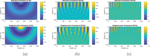
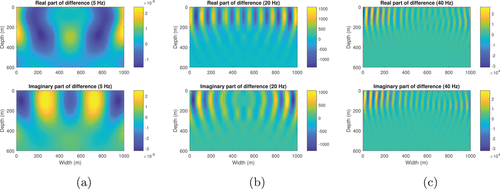
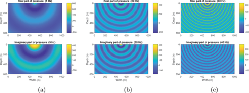
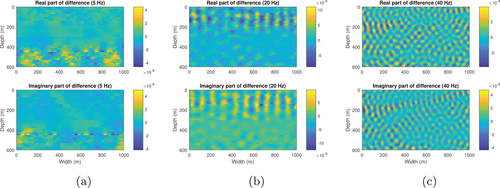
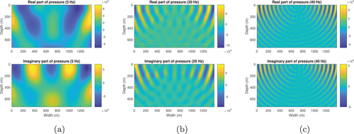
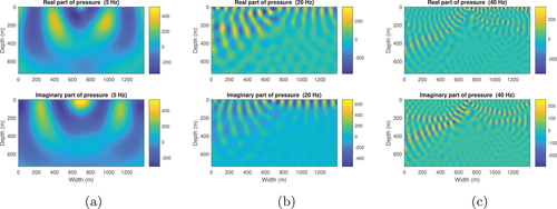
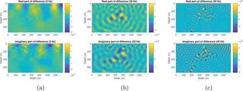
First we calculate wavefields in the three-layer model (Fig. 3). The size of this model is 1000 m wide and 600 m deep. The discrete grid size of the real-space in horizontal and vertical direction are both 10 m. Ideally the space grid should go to 0, but that is not necessary. So usually we choose the grid spacing interval smaller than 1 / 4 of the smallest wavelength λ min , which means the grid spacing interval should smaller than v min / 4 f max . The number of grid blocks is N = 100 × 60 = 6000 . Figure 4 shows reference wavefields of different frequencies calculated by matrix inversion (18). Figure 5 shows the real and imaginary part of wavefields at different frequencies obtained from the Born series. Figure 6 shows the differences between Born-series wavefields and reference wavefields at different frequencies. Figure 7 shows wavefields at different frequencies obtained from the homotopy series. Figure 8 shows the differences between homotopy-series wavefields and reference wavefields at different frequencies. We also computed the normalized overall difference to quantify the convergence performance of the Born series and homotopy series. Figure 9 shows the normalized overall difference changes with iterations for the Born series. Figure 10 shows the normalized overall difference as a function of iteration for the homotopy series. From Figures 4-10, we can see:
  • 1. The wavefields from the homotopy series matches well with the reference wavefields at all frequencies;
  • 2. The Born series only converges at very low frequencies;
  • 3. The homotopy series still converges when the Born series diverges;
Details are in the caption following the image
The three-layer model and its background model.
Details are in the caption following the image
Reference wavefields at (a) 5 Hz, (b) 20 Hz and (c) 40 Hz via matrix inversion within the three-layer model in Figure 3
Details are in the caption following the image
Wavefields at (a) 5 Hz, (b) 20 Hz and (c) 40 Hz via Born series within the three-layer model in Figure 3.
Details are in the caption following the image
Differences between the Born-series wavefields and the reference wavefields at (a) 5 Hz, (b) 20 Hz and (c) 40 Hz within the three-layer model in Figure 3.
Details are in the caption following the image
Wavefields at (a) 5 Hz, (b) 20 Hz and (c) 40 Hz via homotopy series within the three-layer model in Figure 3.
Details are in the caption following the image
Differences between the homotopy-series wavefields and the reference wavefields at (a) 5 Hz, (b) 20 Hz and (c) 40 Hz within the three-layer model in Figure 3.
Details are in the caption following the image
Normalized overall differences versus iteration for Born series at (a) 5 Hz, (b) 20 Hz and (c) 40 Hz within the three-layer model in Figure 3.
Details are in the caption following the image
Normalized overall differences versus iteration for homotopy series at (a) 5 Hz, (b) 20 Hz and (c) 40 Hz within the three-layer model in Figure 3.

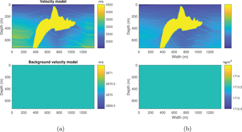
Next we calculate the wavefield in the resampled SEG/EAGE salt model (Fig. 11). The density of this model (Fig. 11b, upper) apart from the salt dome portion is obtained from velocity (Fig. 11a, upper) by Gardner's relation: ρ = 230 v 0.25 (Gardner et al., 1974). The density of the salt dome portion is set equal to the density of halite, which is 2160 kg/m 3 (Mavko et al., 2009). The size of this model is 1390 m wide and 740 m deep. The grid size of each discrete point is 10 m × 10 m. The number of grid blocks is N = 139 × 74 = 10 , 286 . Figure 12 shows the reference wavefield obtained via matrix inversion at different frequencies. Figures 13 and 15 show the wavefield at different frequencies via the Born series and the homotopy series. Figure 14 and  16 show the differences for Born and homotopy series at different frequencies. Figures 17 and 18 present the convergence performance of the Born series and the homotopy series. Clearly, we see that the wavefield from homotopy series is similar to the reference wavefield and the normalized overall difference becomes very small after up to 45 iterations while the wavefield produced using the Born series is totally different from the reference wavefield, and the normalized overall difference diverges in all frequencies.
Details are in the caption following the image
The resampled SEG/EAGE salt model and its background model.
Details are in the caption following the image
Reference wavefields at (a) 5 Hz, (b) 20 Hz and (c) 40 Hz via matrix inversion within the resampled SEG/EAGE salt model in Figure 11.
Details are in the caption following the image
Wavefields at (a) 5 Hz, (b) 20 Hz and (c) 40 Hz via Born series within the resampled SEG/EAGE salt model in Figure 11.
Details are in the caption following the image
Differences between the Born-series wavefields and the reference wavefields at (a) 5 Hz, (b) 20 Hz and (c) 40 Hz within the resampled SEG/EAGE salt model in Figure 11.
Details are in the caption following the image
Wavefields at (a) 5 Hz, (b) 20 Hz and (c) 40 Hz via homotopy series within the resampled SEG/EAGE salt model in Figure 11.
Details are in the caption following the image
Differences between the homotopy-series wavefields and the reference wavefields at (a) 5 Hz, (b) 20 Hz and (c) 40 Hz within the resampled SEG/EAGE salt model in Figure 11.
Details are in the caption following the image
Normalized overall differences versus iteration for Born series at (a) 5 Hz, (b) 20 Hz and (c) 40 Hz within the resampled SEG/EAGE salt model in Figure 11.
Details are in the caption following the image
Normalized overall differences versus iteration for homotopy series at (a) 5 Hz, (b) 20 Hz and (c) 40 Hz within the resampled SEG/EAGE salt model in Figure 11.

Table 2 shows the computational time of different method for different models and frequencies. From Table 2, we see: (1) Matrix inversion is the most time-consuming method; (2) In the case of convergence, Born series is the least time-consuming; (3) Born series only converges at low frequencies in low contrast model; That is because even if the contrast of density or the bulk modulus is very small, putting them together will make the entire contrast arise; (4) Homotopy series not only guarantees convergence in all cases, it also takes much less time than matrix inversion; (5) The larger the model, the more time homotopy series saves compared to matrix inversion. All experiments are performed on an computer with an Intel i7-7700, a 3.6 GHz CPU and a 64 GB RAM.

Table 2. Computational time of different methods
The three-layer model The resampled SEG/EAGE salt model
Frequency 5 Hz 20 Hz 40 Hz 5 Hz 20 Hz 40 Hz
Matrix inversion 111 s 117 s 111 s 589 s 675 s 606 s
Born series 8 s diverge diverge diverge diverge diverge
Homotopy series 23 s 30 s 43 s 77 s 145 s 227 s

CONCLUSIONS

We have derived a vectorial integral equation of the Lippmann-Schwinger (LS) type for seismic forward modelling in acoustic medium with variable velocity and density. This vectorial LS equation is derived from two coupled integral equations. In order to solve it efficiently, we have introduced the homotopy analysis method. The homotopy series is obtained after solving the vectorial LS equation with the homotopy analysis method. It is more flexible than the conventional Born series due to the introduction of the convergence control operator H. We have analysed that if H approximates ( I G ( 0 ) V ) 1 , the homotopy series will converge. Based on this, we constructed the convergence control operator H by using low-rank matrix approximation and hierarchical matrices.

On the basis of the numerical experiments, we have compared the performance of homotopy series with conventional Born series and matrix inversion. Compared with the conventional Born series, the corresponding homotopy series assures convergence in high contrast media and for high frequencies. Compared with matrix inversion, the homotopy series reduces the scale of computational cost from N 3 to N 2 , where N is the number of grid blocks. Numerical examples also show that the larger the model, the more computational time is reduced. This makes our approach suitable for the application of realistic large problems.

This paper mainly focuses on providing a new perspective for seismic forward modelling with variable density and velocity. In future work, an investigation of the optimal form of the hierarchical matrices for constructing convergence control operators as well as the use of Fast Fourier Transform in the construction of the hierarchical matrices (Eikrem et al., 2020) should be included. Also, it might be interesting to use the vectorial LS equation and its homotopy series solution for simultaneous inversion of velocity and density.

ACKNOWLEDGEMENTS

The authors acknowledge the China Scholarship Council for the financial support for Kui Xiang study in Norway. Eikrem, Nævdal and Jakobsen would like to acknowledge the Research Council of Norway (RCN) for the Petromaks II project 267769 (Bayesian inversion of 4D seismic waveform data for quantitative integration with production data) and the National IOR Centre of Norway and its industrial partners, ConocoPhillips Skandinavia AS, Aker BP ASA, Vår Energi AS, Equinor ASA, Neptune Energy Norge AS, Lundin Norway AS, Halliburton AS, Schlumberger Norge AS and Wintershall DEA for support. We are also very grateful to the reviewers and editors for their effort and patience in reviewing this manuscript.

    APPENDIX

    3D GREEN'S FUNCTION AND ITS SPATIAL DERIVATIVES

    The three-dimensional acoustic Green's function for a homogeneous medium in the frequency domain can be expressed as (Červený, 2005)
    G ( 0 ) ( r , ω ) = 1 4 π r exp ( i ω r / c 0 ) , (A1)
    where
    r = x x , r = r . (A2)
    For the convenience of derivation, we introduce the following notation:
    A ( r ) = 1 4 π exp ( a r ) , Z ( r ) = r , a = i ω / c 0 . (A3)
    Equation (A1) can be rewritten as
    G ( 0 ) ( r ) = A ( r ) Z ( r ) . (A4)
    From (A1)–(A4), we have
    x G ( 0 ) = G ( 0 ) x = G ( 0 ) r r x , (A5)
    A r = a A , Z r = 1 , (A6)
    G ( 0 ) r = ( A / r ) Z A ( Z / r ) Z 2 = a A Z A Z 2 , (A7)
    r = r = r T r = l , (A8)
    l = r T r = ( x x ) T ( x x ) = ( x T x 2 x T x + x T x ) , (A9)
    l x = 2 ( x x ) = 2 r , r l = 1 2 r , (A10)
    r x = r l l x = 1 r r . (A11)
    By combining (A3), (A5), (A7) and (A11), we obtain the first spatial derivatives of G ( 0 ) :
    x G ( 0 ) ( r , ω ) = A a Z 2 1 Z 3 r = 1 4 π exp ( i ω r / c 0 ) i ω c 0 r 2 1 r 3 r . (A12)
    From (A12), we write the second spatial derivative of G ( 0 ) as
    x x G ( 0 ) = x G ( 0 ) x = a x A Z 2 r x A Z 3 r . (A13)
    According to (A2), we derive
    r x = I 3 , (A14)
    where I 3 is a 3 ×3 identity matrix. In (A13), we have
    x A Z 2 r = x A Z 2 r + A Z 2 r x = a A Z 2 2 A Z Z 4 r x r + A Z 2 I 3 , (A15)
    x A Z 3 r = x A Z 3 r + A Z 3 r x = a A Z 3 3 A Z 2 Z 6 r x r + A Z 3 I 3 . (A16)
    By combing (A3), (A13), (A15) and (A16), we obtain the second spatial derivatives of G ( 0 ) :
    x x G ( 0 ) ( r , ω ) = A a 2 Z 3 3 a Z 4 + 3 Z 5 r r T + a Z 2 1 Z 3 I 3 = 1 4 π exp ( i ω r / c 0 ) ω 2 c 0 2 r 3 3 i ω c 0 r 4 + 3 r 5 r r T + i ω c 0 r 2 1 r 3 I 3 . (A17)

    2D GREEN'S FUNCTION AND ITS SPATIAL DERIVATIVES

    The two-dimensional Green's function for a homogeneous acoustic medium is (Červený, 2005)
    G 2 D ( 0 ) ( r , ω ) = 1 4 i H 0 ( 1 ) ( ω r / c 0 ) , (B1)
    where
    r = x x , r = r (B2)
    and H 0 ( 1 ) is the Hankel function of the first kind and zeroth order. The Hankel function has the recurrence relation (Arfken and Weber, 1999):
    H 0 ( 1 ) ( x ) x = H 1 ( 1 ) ( x ) , 2 H 0 ( 1 ) ( x ) x 2 = H 0 ( 1 ) ( x ) + H 1 ( 1 ) ( x ) x . (B3)
    We introduce a new notation:
    Z ( r ) = ω r / c 0 . (B4)
    From (B2), we derive
    r x = 1 r r , r x = I 2 , (B5)
    where I 2 is a 2 ×2 identity matrix.
    According to the chain rule and (B1)–(B5), we get
    x G 2 D ( 0 ) ( r , ω ) = G 2 D ( 0 ) x = G 2 D ( 0 ) H H Z Z r r x = i ω 4 c 0 r H 1 ( 1 ) ( ω r / c 0 ) r . (B6)
    Through (B5), we obtain
    2 r x 2 = x r x = x r r = ( r / x ) r r ( r / x ) r 2 = 1 r I 2 1 r 2 r r T . (B7)
    By using the chain rule and (B3)–(B7), we have
    x x G 2 D ( 0 ) ( r , ω ) = x G 2 D ( 0 ) x = i ω 4 c 0 x H Z r x = i ω 4 c 0 2 H Z 2 Z r r x r x + H Z 2 r x 2 = i ω 4 c 0 1 r H 1 ( 1 ) ( Z ) I 2 + ω c 0 r 2 H 0 ( 1 ) ( Z ) + H 1 ( 1 ) ( Z ) Z + 1 r 3 H 1 ( 1 ) ( Z ) r r T = i ω 4 c 0 1 r H 1 ( 1 ) ( ω r / c 0 ) I 2 + ω c 0 r 2 H 0 ( 1 ) ( ω r / c 0 ) + 2 r 3 H 1 ( 1 ) ( ω r / c 0 ) r r T . (B8)

    DATA AVAILABILITY STATEMENT

    The data that support this study are available from the corresponding author on reasonable request.

      The full text of this article hosted at iucr.org is unavailable due to technical difficulties.