Simulating geophysical models through fractal algorithms
ABSTRACT
I present an algorithm, borrowed from the computer graphics industry, that is able to efficiently and effectively simulate pseudo-realistic topographies and three-dimensional geophysical models. It has been widely exploited in the movie industry for generating artificial landscapes and for simulating the surface of planets. The geophysical applications are manifold: simulation for testing inversion algorithms, interpolation, and upscaling are only some of the possibilities.
INTRODUCTION
Since the 1970s, when Mandelbrot presented first applications (Mandelbrot 1971), the subject of fractals has attracted interest throughout several disciplines, including engineering, medicine, economics, and social science to name a few. Barnsley (1993) introduced new concepts, like the collage theorem, and new algorithms, like the iterated function system, and showed that any natural shape can be reconstructed through a fractal algorithm. It is now well understood that classical modelling techniques exploiting Euclidean geometry, such as prism-based or tetrahedral-based modelling, are well suited more for describing man-made structures than natural shapes. The aforementioned paper from Mandelbrot was actually a geophysical application. We could now count an endless number of applications of fractal techniques to geophysics. Pilkington and Todoeschuck (2004) studied the fractal distribution of real crustal density sources and related this distribution to the shape of the power spectrum of 2D density slices. Maus and Dimri (1994) proposed how to derive fractal parameters of the subsurface density distribution from the estimated fractal parameters of surface gravity data. The interested reader is referred to Turcotte (1997) for having numerous examples and references for geophysical applications.
Whenever any scientist develops a new algorithm, he will need to perform several tests for assessing its stability, reliability, and robustness. The algorithm should also be tested on real cases in order to verify its effectiveness. For this reason, it would be convenient to have a method for simulating realistic cases automatically so that thousands of tests could be automatically performed and reliable conclusions could be drawn from the statistical analysis of the outcomes. This is the main motivation that drove the research of a method for automatically generating realistic topographies and geophysical models.
If we look at the state of the art of the algorithms currently exploited in the industry of computer graphics, we understand that the level of such technology is far beyond what it has been exploited up to now in geophysics. In 1980, Loren Carpenter presented for the first time one of the most successful techniques for the generation of synthetic topographies: the diamond-square algorithm (Carpenter 1980). Carpenter's presentation was met by a real standing ovation, and he was then hired by Lucasfilm's computer science division (now Pixar) for the realisation of the Genesis effect for the movie titled Star Trek II: The Wrath of Khan. The details and possibilities of this algorithm are well explained in Fournier, Fussell and Carpenter (1982), where the authors show the simulation of realistic coastlines, landscapes, and planet surfaces.
In this paper, I review the basics of the diamond-square algorithm and I show an extension I devised for the automatic generation of 3D geophysical models. Before doing this, in order to keep this paper as much self-contained as possible, I will review some fundamental concepts on the mathematics of fractals because they are necessary for understanding the mechanics of the geophysical simulation algorithm.
FUNDAMENTALS ON FRACTALS
The most important property of a fractal is self-similarity, which means that the object is similar to itself at all scales. Figure 1 shows the self-similarity using the Julia set as an example. Figure 1a shows the Julia set with a highlighted rectangular region. Figure 1b shows the zoomed rectangle in Fig. 1a brought at the same scale as the previous image. It is now clear what self-similarity means (rotations are allowed).

 (1)
(1) is the total number of elements with characteristic linear dimension
  , C is a proportionality constant depending on the fractal itself, and D is the fractal dimension.
The fractal dimension itself is a very important parameter and must be fully understood for being able to appreciate its information and the contribution it has in the simulation algorithm explained later. For this reason, although the main objective of this paper is not a dissertation on the fractal dimension, I will explain some basic concepts and I will also provide hints on how this parameter can be estimated1.
The fractal dimension is basically a measure of the random nature of the fractal. Also, it is greater or equal to the topological dimension and, usually, lower than the Euclidean dimension2. The Euclidean dimension is a non-fractal dimension, and it is simply given by the number of coordinates required for describing a geometrical object. The rigorous definition of the topological dimension is more involved and would require more space than what is reasonable for this paper. The interested reader is referred to Barnsley (1993) and to Addison (1997). On the other hand, it is easy to get an intuitive understanding of the topological dimension. Consider, for example, to be an insect moving on the space of our geometrical object. We can count the number of degrees of freedom of possible movements, and that number is the topological dimension. To have some useful examples, a curve in the 3D space has a topological dimension of one but a Euclidean dimension of three. A surface in the space has a topological dimension equal to two and a Euclidean dimension of three. A point has both the topological and Euclidean dimensions equal to zero. Further examples of Euclidean and topological dimensions are given in Addison (1997).
 (2)
(2) (3)
(3) sides, each of length
  . In Fig. 2b, we count
  sides, each of length
  . By applying expression 3, we find

As explained above, this value is larger than the topological dimension of the coastline, which is one, and smaller than the Euclidean dimension, which is two. The reader is invited to verify that the same result is obtained by using Fig. 2b and c. Also, the reader can easily verify that the fractal dimension of non-fractal objects, like a square or a segment, is always equal to their topological dimension. For this reason, we understand that the fractal dimension is also a measure of how much the fractal is able to fill the space described by the Euclidean dimension. Fractals that have a fractal dimension larger than the Euclidean dimension are filling the space more than the Euclidean dimension and are typically geometrical objects that “fold on themselves” maybe many times (Barnsley 1993; Addison 1997).

- Similarity dimension It is the dimension provided by using equation 3 and has the drawback that, in order to compute it, we need to identify exactly self-similar parts of the fractal. It cannot be used for estimating the fractal dimension of statistical fractals, which are those we are interested in, because these are those through which we can simulate natural objects (as we will see later).
- Hausdorff dimension It is the most rigorous fractal dimension definition but it has little practical use because of the difficulty of its estimation. Its definition is out of the scope of this paper, and the interested reader is referred to Barnsley (1993).
- Box-counting dimension Explained into the Appendix of this paper, this provides a good approximation of the Hausdorff dimension. It is the most useful because it is easy to estimate and can be applied also to statistical fractals and natural fractals (e.g., topographies, coastlines, and pore distributions in rocks).
SELF-AFFINE FRACTALS
 (4)
(4) and
and  .
.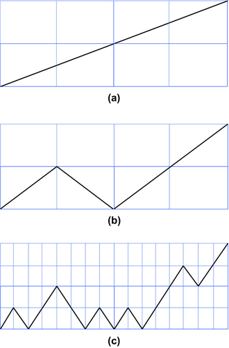
 and
and  .
. (5)
(5) is the topological dimension. Despite its simplicity, as the proof of equation 5 would be too lengthy to describe here, the interested reader is referred to Turcotte (1997). Another interesting property of equation 5 is that it is valid also for fractals that contain randomness (i.e., statistical fractals). For this reason, it is extremely useful for simulating natural shapes, as we will see in the following.
SIMULATING TOPOGRAPHIES
Topographies or bathymetries can be very well approximated by a fractional Brownian process (Addison 1997), which is nothing more than a statistical self-affine fractal. In computer graphics, topographies and bathymetries are simulated as fractal landscapes, and the widely used technique for their simulation is the well-known diamond-square algorithm (DSA), described in detail by Fournier et al. (1982). Figure 4 shows the basic steps performed by the algorithm. We start with a square grid, with a number of samples that is a power of 2 plus one on each side. Each iteration of the algorithm is composed of two steps: the diamond step and the square step.
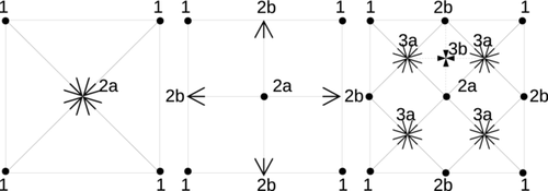
 the single sample of our 2D signal, at row i and column j, the computation performed is
 (6)
(6) is additive white Gaussian noise (AWGN) with zero mean and unitary standard deviation;
  multiplies the AWGN term and is often referred to as roughness.
 (7)
(7) (8)
(8) for the initial roughness. Because these are fractals, we could assign any length to the side of the square grid and scale the initial roughness accordingly, without modifying the final result. No a priori information has been used for the simulation. The initialisation of the grid was simply done by setting to zero the four corners. It is clear that, when the Hurst exponent increases, the fractal dimension decreases, according to equation 5, where we need to set
  . The higher the fractal dimension, the higher is the level of chaos shown by the fractal. The more realistic topography results are those shown in Fig. 5b and c because the average Hurst exponent of real topographies on the Earth is around
  (Addison 1997). Furthermore, notice that the topography in Fig. 5d has a fractal dimension
  , which is smaller than its topological dimension (
 ), and for this reason, it is not properly a 2D object.
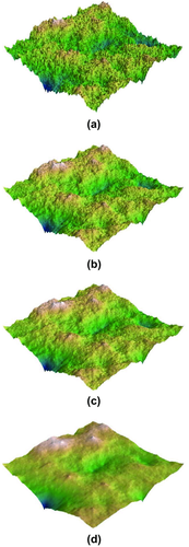
 ; (b)
; (b)  ; (c)
; (c)  ; and (d)
  .
.SIMULATING THREE-DIMENSIONAL PROPERTY VOLUMES
The possibility to simulate geophysical models through fractal techniques is not new. Srivastava and Sen (2010) show how to simulate reservoir models with a frequency-domain fractal algorithm. This approach has the disadvantage that it cannot be seeded with known values in the space domain. For this reason, I preferred the diamond-square algorithm (DSA) that is equivalent to the frequency-domain approach, like is demonstrated by Fournier et al. (1982), and that can be seeded with known values in the space domain.
The DSA can be trivially extended to handle the simulation of 3D property volumes. Figure 6 shows the basic steps to perform. For readability, the cube in the middle shows only the computations on two of the six faces of the cube. Similarly, the cube on the right shows the computation that needs to be performed for updating the midpoint of only one of the 12 sides of the cube. At each pass on the cube, similarly to what is done for the 2D DSA, the algorithm will operate on a halved scale and will reduce the roughness again through the application of equation 8. Blindly applying this 3D algorithm with no a priori information will hardly produce a realistic geophysical model. In this case, it is necessary to drive the algorithm towards a geophysical solution by exploiting the possibility to initialise some samples upfront.

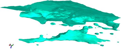
Figure 7 shows the result of a simulation performed using a subset of the samples of the SEG Advanced Modeling program (SEAM) density model as the seed for the 3D DSA. I first initialised a 129 × 129 × 129 empty grid by taking one sample every 16 from an equally sized region of the SEAM model. No anti-aliasing filter was applied before downsampling because, in this application, the objective is to exploit aliasing. Then, I ran the 3D version of the DSA on this grid. Figure 7 shows, on the left, a cross section of this portion of the SEAM model and, on the right, the same cross section taken from the simulated model. We clearly see that the algorithm was able to generate a synthetic model that is sufficiently different from the original one and that, at the same time, presents interesting pseudo-realistic features such as the salt. Even if this model does not have the same resolution as the original one, it is suited to be used for testing forward modelling and inversion algorithms. The realistic features of this synthetic model are even more evident from Fig. 8, which shows an isosurface taken at 2250 kg/m3.

 .
.
CONCLUSIONS
I have presented an efficient and effective technique for generating pseudo-realistic synthetic topographies and geophysical models. This technique is well known in the computer graphics industry as the diamond-square algorithm (DSA). It can be used to produce synthetic topographies also with no a priori information. Realistic 3D geophysical models can be produced by exploiting some a priori information coming from existing real or synthetic but realistic models. The degree of similarity with the a priori model can be freely chosen by the user. The possible applications of the algorithm are manifold: modelling and simulation, interpolation, upscaling, and exploitation in algorithm robustness assessment are only some of the many possibilities. In De Stefano and Panepinto (2016), I exploited this algorithm for quantifying the topographic staircase effect caused by poor sampling of the topography when using right rectangular prisms in potential field modelling. Numerical simulations with a reasonable choice for the Hurst exponent allowed me to provide practical suggestions for the choice of the most appropriate sampling interval.
Although I extended the DSA to the simulation of fractal property volumes, I want to stress that the original algorithm was devised explicitly for producing fractal surfaces, which can also be closed. In Fournier et al. (1982), the authors show how they are able to realistically simulate the closed surface of a planet. For this reason, it is possible, by choosing the right fractal parameters, to simulate also the closed surface of a salt body or generally any geophysical, multi-valued, surface. Such a development could lead to other interesting applications, for example, examining the reflection phase and amplitude response of seismic data as a function of surface roughness. This is of particular interest for velocity (or other parameter) model building, especially if we are using dynamic information to drive the inversion, such as is the case in waveform inversion. At what scale length of roughness, as a function of dominant seismic frequency, does roughness become important?
A warning must be raised for the exploitation of this method, as is, for the creation of model realisations for geostatistical analysis or Bayesian uncertainty estimation. For such applications, it would be invalid to blindly create fractally perturbed model distributions unless the so-derived models are checked with some additional technique for their acceptability as a valid solution of the inverse problem. More research needs to be done in this field.
ACKNOWLEDGEMENTS
The author would like to thank Schlumberger for having allowed the publication of this paper. The author would also like to thank EAGE for having been invited to transform this subject from a conference extended abstract into what is seen here. Many thanks to the author's high school mathematics professor, Franco Colombo (Liceo Scientifico di Gallarate, Italy), for having the author introduced to the wonderful world of fractals. The author would also like to thank Mr. Ian Jones and an anonymous reviewer for their suggestions that improved the shape of this paper. In particularly, Mr. Jones is acknowledged for the suggestion of expanding the conclusions about possible applications in the field of waveform inversion and for suggesting to point out the limitations of this technique, as is, if exploited in Bayesian inversions.
APPENDIX: DISCOVERING THE FRACTAL DIMENSION OF NATURAL SHAPES
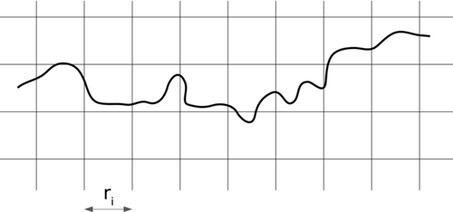
One of the basic steps needed to simulate a natural fractal through the diamond-square algorithm (DSA). is to estimate the Hurst exponent of the real object under examination. It should be clear to the reader that only knowing the best Hurst exponent to use we can effectively obtain a realistic object. The Hurst exponent plays a key role into the reduction of the roughness iteration after iteration (equation 8) and it can be derived once we know the value of the fractal dimension (equation 5). I will now show how the fractal dimension of a natural object can be easily estimated by exploiting the box-counting dimension algorithm. As previously explained in this paper, this estimate is actually the box-counting dimension and it is a very good approximation of the Hausdorff dimension, which is the most rigorous fractal dimension estimate. Once the fractal dimension is known, if we suspect that we are dealing with a fractional Brownian motion, the Hurst exponent can then be derived by using equation 5. A hint we are dealing with a fractional Brownian motion is provided by the  decay of the power spectral density (Turcotte 1997).
 . We then count the number of squares that is crossed by the profile: let us call this number
  . We then perform another iteration, where we reduce the size of the squares. Let us call this new side length as
  . We count again the number of squares that is crossed by our profile. This number is now
  . We can repeat these steps as many times as we want, collecting the
  pair at each iteration k. Now, recall the scale invariance property in equation 1. By taking the logarithm (in any base of choice) on both sides of equation 1, we have
 (9)
(9)
This is a straight line in the log–log space. For this reason, the C and D constants can be estimated by a simple linear regression. This algorithm is applicable also for surfaces by substituting the 2D grid of squares with a 3D grid of cubes. It can also be extended to higher dimensional objects, but if we suspect the fractal to be well approximated by a fractional Brownian motion, we can estimate the fractal dimension of one (or some) 2D or 1D section and then derive the fractal dimension of the whole object. This is possible because any section of a fractional Brownian motion is again a fractional Brownian motion with the same Hurst exponent (Addison 1997). For this reason, we can estimate the fractal dimension of lower dimensional sections (e.g., as the average of the estimate from several sections). This fractal dimension will obviously be lower than the fractal dimension of the whole object but it will have the same Hurst exponent, which is the real parameter we are interested in, because it is this parameter that we provide to the DSA. Once we know the fractal dimension of the lower dimensional section, we exploit equation 5 for deriving the Hurst exponent.


