From noise correlation to resonant ultrasound spectroscopy in rock acoustics

2.1 Laboratory conventional methods to measure elastic constants of a sample

There are three conventional methods for measuring the elastic constants of a solid sample in the laboratory (e.g., Bourbié, Coussy and Zinszner 1987).

The first one is the pulse transmission (PT) method that uses P-wave or S-wave piezoelectric transducers as the source and receiver. The spectrum of the pulse transmitted through the sample is in the ultrasonic frequency band (from a few hundreds of kilohertz to a few megahertz). Knowing the length L of the sample, the measured arrival time t allows us to deduce the wave speed , and the corresponding elastic modulus (the density being independently measured). V designates either the P-wave velocity or the S-wave velocity, i.e.,

(1)

and

(2)

where μ is the shear modulus, K the bulk modulus, and ρ the density of the constituent material.

The second conventional method for measuring elastic constants is the resonant bar method (e.g., Lucet 1989; Lucet, Rasolofosaon and Zinszner 1991). The sample vibrates in the sonic frequency band (a few kilohertz to a few tens of kilohertz). The diameter of the bar should be as small as possible compared with its length, in order to approximately deal with a 1D problem. Classically, by exciting the torsional mode (respectively, the extensional mode) (Fig. 1), one can measure the shear modulus (respectively, the Young's modulus) of the constituent material through the measurement of the resonance frequencies of the lowest modes (e.g., Bourbié et al. 1987). The relation between the length L of the bar, its velocity V, the resonance frequencies (n being the mode number), and the wavelength Λ is given by

(3)

Note that V can designate either the extensional mode velocity ( being the Young's modulus), or the torsional/shear velocity (). Concerning the flexural modes, the relation is a bit different (Bourbié et al. 1987).

The third conventional method consists in forcing vibrations of the sample through a low-frequency dynamic press (e.g., Spencer 1981; Hofmann 2006). A sinusoidal stress is applied by a solenoid-driven shaker to a column composed of a rock sample and end caps made of a standard material, usually aluminium. The resulting sinusoidal deformation and strain is measured by strain gauges mounted vertically and horizontally on the aluminium standard sample and on the rock sample. The stress–strain plots for the rock sample allow one to compute Young's modulus and Poisson's ratio. The corresponding plots for the standard aluminium (of known elastic properties) are used to calibrate the method.

The frequency range concerns the seismic frequency band, typically from a few tens of hertz to a few hundreds of hertz.

2.2 Resonant ultrasound spectroscopy

RUS is a laboratory technique used in the communities of Geophysics and Material Science for measuring elastic properties of solids (e.g., Maynard 1996; Migliori and Sarrao 1997). It consists in forcing the mechanical resonance of a solid sample and inverting the measured natural resonance frequencies of the sample in terms of the elastic moduli of the constituent material (Fig. 2). Note that the resonant bar method can be considered a very special case of the RUS method, where the resonating solid is one-dimensional. However in a conventional RUS experiment, the sample can have more complicated shape such as spherical (Anderson et al. 1970), cubic (Demarest 1971), parralelepipedic (Ohno 1976), or even arbitrary shape (Visscher et al. 1991).

The first RUS experiment was performed by Fraser and LeCraw (1964) on an isotropic sphere. The measured resonance frequencies were graphically inverted using the analytic solution of the problem for an isotropic elastic sphere, found around 1880 by Lamé and Lamb (e.g., Maynard 1996).

In a RUS experiment, the operator imposes the vibration frequency sent to the sample of arbitrary but known shape and dimension. Each frequency ω is sent one by one, and the induced displacement U(t) is measured (Fig. 2). Thus, the root-mean-square value of U as a function of the frequency (the resonance spectrum of the sample) can be plotted. Finally, the elastic constants C_ijkl are deduced from the picked resonance frequencies, the geometry, and the density of the sample.

3.1 The experimental setup

Figure 3 shows the experimental setup corresponding to an ultrasound spectroscopy experiment using random-noise excitation.

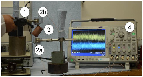
The sample is a cylinder, which is about a decimetre long and roughly half a decimetre wide. For simplicity, we exploited only this simple geometry. However, as previously pointed out, in principle, any alternative but known geometry could have been chosen. The frequency band of the source is about a few 10⁴ Hz, and P-wave and S-wave velocities are about a few kilometres per second.

Consequently, wavelengths are about a ten of centimetres, which is the average sample length. Thus, resonance regime dominates wave propagation regime. For further consideration on this topic, the reader can refer to the work of Bourbié et al. (1987, Sec. 3.5.1) on “travelling waves and vibrations.”

The sample is placed between two passive piezoelectric sensors, in a way that minimizes the contact surface. In fact, the ideal situation would be point contacts, to permit free vibrations of the sample.

The sensors are plugged to an oscilloscope that records the signals.

We generate noise into the sample by means of a pneumatic air blow gun (here after simply called “air blow gun”). In this way, this experiment is a bit different from a classical RUS experiment as we do not control the emitted frequency.

Four samples are used in this study. The first one is a cylinder (diameter D = 6 cm and length L = 10 cm) of aluminium, more precisely, a common commercial alloy of aluminium (>90%), copper (3% to 5%), manganese (0.3% to 1%), and magnesium (0.4% to 2.4%) called duralumin. The second sample is a cylinder (D = 6 cm and L = 10 cm) of Plexiglas, which is a homogeneous and attenuating material. The two last samples are cylinders of the same dimension (D = 4 cm and L = 8 cm) made of rock, namely Vilhonneur limestone and Euville limestone.

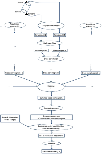
3.2 The workflow

3.3 Signal processing before resonance peak identification

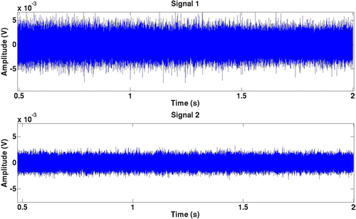
Figure 5 shows a pair of raw signals acquired with an aluminium cylinder. We can observe correlated events, coming from fortuitous noisy events in the laboratory. These low-frequency events (with frequency smaller than 5 kHz) are generated by a fan or another running machine.

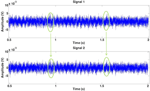
Consequently, we apply a 5-kHz high-pass filter to randomize the signals. Of course, we choose the lowest cut-off frequency allowing us to keep as much information as possible. This step helps us to comply with the equipartition condition, i.e., the best condition for doing noise correlation (e.g., Schuster 2009). Figure 6 shows the same pair of signals after filtering. Note that the low-frequency coherent arrivals shown in Fig. 5 have disappeared.

The next step is about the summation (or “stacking”) of the cross-correlations.

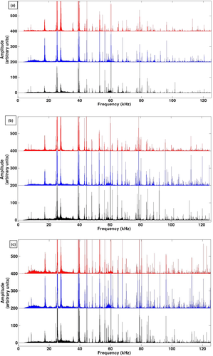
Figure 7 represents the spectra of three different single cross-correlations. Even if these spectra are close to each other, we clearly observe that specific resonant peaks are present in the spectrum of a cross-correlogram and not in another one. Figure 8 represents the spectrum of three different sets of 5 (Fig. 8a), 10 (Fig. 8b), or 15 (Fig. 8c) cross-correlations stacked together. A given individual cross-correlogram belongs only to one set of N_stack (= 5, 10, or 15, respectively) cross-correlograms. Obviously, the stacking process improves the SNR and provides a stable and reproducible signal (in terms of resonance frequency list) if N_stack is greater than 10, as far as aluminium sample is concerned. As a consequence,

we decide to sum together 15 cross-correlations (N_stack = 15) acquired on an aluminium sample. In the case of more attenuating samples, as Plexiglas, the required number of cross-correlations to be stacked in order to stabilize the spectrum is 40 (N_stack = 40).

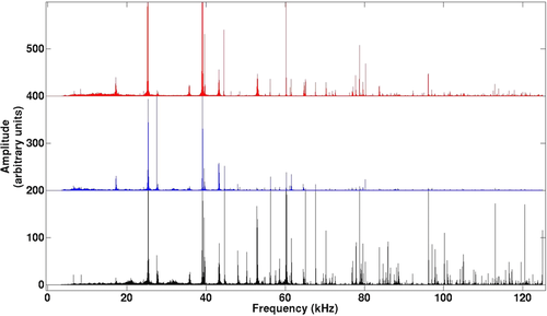
The experiment deals with resonance modes. It is then interesting to compare the difference between: (i) the spectrum obtained from cross-correlation of signals recorded at both sensors; (ii) the spectra obtained from auto-correlation of signals recorded at each sensor; and (iii) the spectra of the raw signals (Figs. 9-12).

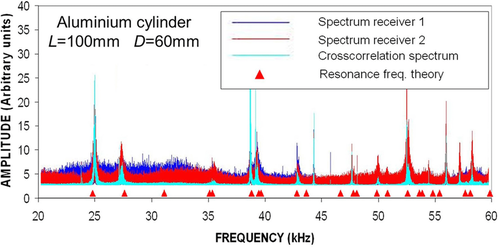
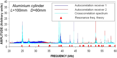
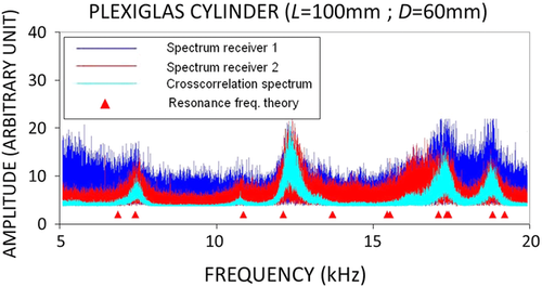
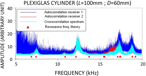
Figures 9 and 11 show the sum of N_stack spectra of the recorded signals on receiver 1 (in blue line), of the recorded signals on receiver 2 (in red line), and the spectrum of the N_stack cross-correlograms (in cyan line), respectively, for the aluminium cylinder (N_stack = 15) and for the Plexiglas cylinder (N_stack = 40). Similarly, Figs. 10 and 12 show the spectra of the N_stack stacked auto-correlograms of the recorded signal on receiver 1 (in blue line), of the recorded signal on receiver 2 (in red line), and the spectrum of the N_stack stacked cross-correlograms (in cyan line), respectively, for aluminium and for Plexiglas. For comparison, we also plot on all these figures the theoretical resonance frequencies (in red triangles) corresponding to the elastic constants independently measured with the conventional ultrasonic pulse transmission (PT) technique.

Much can be said about these figures, but here, we only want to focus on the main results.

First, on non-attenuating samples, here aluminium (Figs. 9 and 10), all the resonance peaks are present in any of the spectra. As the corresponding resonance frequencies are the only inputs for the inversion of the elastic parameters of the solid, any of these curves can be equivalently used for measuring the elastic properties of the tested sample in resonance mode. A possible physical explanation is that the spectrum of the input random source signal is strongly filtered by the resonant cavity constituted by the solid cylinder. As a consequence, any of the spectra of Figs. 9 and 10 are dominated by the resonance peaks of the non-attenuating solid cylinder. However, let us note that the spectrum of N_stack cross-correlograms definitely helps the identification of resonance frequencies because, for instance, the resonance peaks are sharper than the peaks that can be identified on the sum of N_stack spectra of raw signals (see Fig. 9). In contrast, SNRs are comparable on the spectra of 15 stacked auto-correlations (receivers 1 and 2) and on the spectrum of the 15 stacked cross-correlations (see Fig. 10). However, note a slightly lower SNR for the spectrum of the 15 stacked auto-correlations corresponding to receiver 1 (curve in blue line in Fig. 10). In conclusion, we can say that the correlation process (either cross-correlation or auto-correlation) tends to improve the SNR.

In comparison, the contrast is stronger in the case of Plexiglas (see Figs. 11 and 12), due to the impact of attenuation. More precisely, as shown in Fig. 11, the SNR of the sum of 40 spectra of raw signals is so weak that some resonance peaks are hardly visible. This is the case for the resonance peak around 11 kHz for receiver 1 (blue curve in Fig. 11) and for the resonance peak around 18 kHz for receiver 2 (red curve in Fig. 11). As a consequence, from a practical point of view, the sum of 40 spectra of raw signals cannot be safely used to identify the resonance frequencies, as required to invert the elastic parameters of attenuating samples.

In contrast, these peaks are clearly visible on the spectrum of the 40 stacked cross-correlations (cyan curve in Fig. 11). The correlation process strongly improves the SNR, and the result is much more convincing than in the non-attenuating sample (compare Figs. 11 and 9). Furthermore, the resonance peaks are slightly less visible on the spectra of 40 stacked auto-correlations (blue and red curves in Fig. 12) than on the spectrum of the 40 stacked cross-correlations (cyan curve in Fig. 12), particularly on receiver 1 (blue curve in Fig. 12). From a general point of view, the resonance peaks are more visible on receiver 2 (red curve in Fig. 12) than on receiver 1. This may be due to many reasons, for instance, the quality of the receiver transducer itself, the quality of the coupling between the receiver and the solid sample, or the location of the recording point, to name a few. Moreover, whatever the individual quality of the recordings at receivers 1 and 2, it appears that the cross-correlation process seems in some way to make up for the possible low quality of one of the recordings. As a consequence, clear resonance peaks are exhibited, strongly facilitating the inversion of the elastic parameters. As a conclusion, in the presence of attenuation, the cross-correlation process appears to be the most efficient way to track the resonance peaks of a vibrating sample in order to invert the elastic parameters of its solid constituent.

3.4 Resonance-peak identification

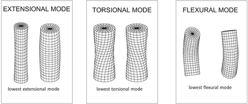
This step is extremely important. It consists in linking each resonance peak to a resonance mode of the sample. As our samples are cylindrical, the main resonance mode families are torsional mode, flexural mode, and extensional mode, as illustrated in Fig. 1. More details can be found in (Meeker and Meitzler 1964).

As explained in Appendix B, the main input of the inversion procedure that we use is an exhaustive list of the resonance frequencies in the frequency band of interest. More precisely, even if a frequency is not present in our experimental spectrum, it has to be present in the list of resonance frequencies. Clearly, in the objective function F to be minimized (i.e., the deviation between the computed resonance frequencies and the measured resonance frequencies), the weight factor for this absent frequency would be zero (see details in Appendix B). In contrast, the weight factor will be one for all the identified frequencies.

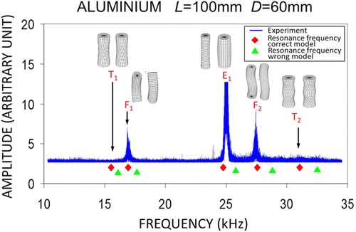
As an illustration, Fig. 13 shows the impact of omitting a resonance frequency in the input list on the inverted model. More precisely, the experimental spectrum of the 15 stacked cross-correlations in an aluminium sample (between 10 kHz and 35 kHz) is plotted in a solid blue line. The solid red diamonds stand for the resonance frequencies linked to P-wave and S-wave velocities obtained from the inversion of all the frequency peaks, including the fundamental torsional mode T₁. This mode is not identified on the experimental spectrum, but its frequency (about 15 kHz) is known by forward modelling using the P-wave and S-wave velocities measured by PT. If we do not include this frequency in the input frequency list, the inversion result is substantially different, namely 1.7% deviation on C₁₁ and 9.7 % on C₄₄. Furthermore, at the end of the inversion process, the final value of the objective function F is much smaller (typically two orders of magnitude) when using the complete list of input resonance frequencies than when omitting even a single frequency (here the resonance frequency of T₁) in the list. In this last case, as expected, the resonance frequencies predicted by the inverted “wrong” model (plotted in solid green triangles in Fig. 13) substantially deviate from the resonance frequencies predicted by the model inverted from the complete list of frequencies (plotted in red solid diamonds in Fig. 13).

3.5 Inversion procedure

We used two codes to compute the resonance frequencies of 3D samples, knowing the dimensions and the elastic constants of the samples.

The commercial software ATILA, based on modal analysis, deals with two or three dimension structures, and it can solve the direct problem and identify the resonance modes.

The free academic software RUS-inverse, developed by Brian Zadler and Jérôme le Rousseau (Zadler et al. 2004) at Colorado School of Mines, is also based on a modal analysis of 3D structures, and can deal with both the direct problem and the inverse problem.

To run the inversion, we used RUS-inverse (see Appendices A and B for details), which requires the shape and the dimensions of the studied sample, an exhaustive list of resonance frequencies, and a priori C₁₁ and C₄₄ values (in the case of an isotropic material).

The importance of the exhaustive list of resonance frequencies has already been discussed. In our case, the a priori elastic constants are measured using another independent experiment, in order to validate our alternative experimental procedure. As a consequence, we measured the first break time for P-wave and S-waves through many samples of the same material and deduced the values of C₁₁ and C₄₄ (see Section 4.3). The results provided by RUS-inverse are a list of the computed resonance frequencies, the computed values of C₁₁ and C₄₄, and the mismatch between the experimental results and the computed results, after the inversion.

4.1 Reproducibility of the experiment

The calibration of the experimental procedure was done with an aluminium cylinder (diameter D = 6 cm and length L = 10 cm).

Figure 14 shows three spectra of a stack of 15 different cross-correlations. For each realization, a different set of 15 correlations is used. We can notice that each resonance frequency remains unchanged from one realization to another. The result is thus quite stable and reproducible. Moreover, when we zoom on a specific resonance peak, for instance, the one at 56,180 Hz, the variation Δf of the resonance frequency from a realization to another is smaller than 7 Hz, which corresponds to a remarkably small relative variation Δf/f of 0.012%.

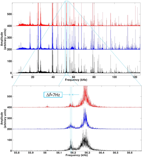
In conclusion, this experiment is highly reproducible.

4.2 Validation of the inversion results

We plot in Fig. 15 the relative difference between the resonance frequency f_UI, corresponding to the model inverted from the experimental resonance curve, and the resonance frequency f_pulse, obtained by forward modelling using the elastic constants independently measured by pulse transmission (PT), as a function of f_pulse in an aluminium sample.

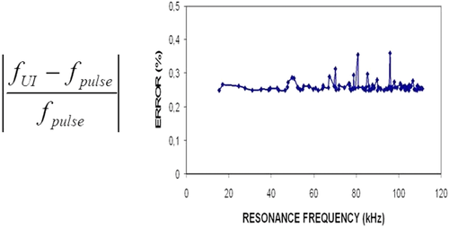
Here again, the average error is quite small, about 0.25%, and thus validates the inversion procedure.

In Section 3.4, we noticed that the code needs a priori elastic constant values of the material studied to initiate the inversion process. For instance, these values can be independently obtained by PT. For this, we choose a set of six aluminium cylinders of different lengths, i.e., 35 mm, 38 mm, 50 mm, 60 mm, 70 mm, and 80 mm (Fig. 16) and machined from a single solid block. We measured the first-arrival time break for P-wave and S-wave through each cylinder. Then, using linear regression, the P-wave and S-wave velocities are obtained, with a high accuracy, as shown in Fig. 17 (typical correlation coefficients are as high as 0.9997 in both cases).

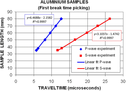
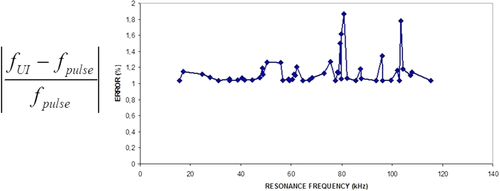
This very precise measurement of the elastic constants by conventional pulse-transmission technique explains the small error we obtain when comparing f_pulse with f_UI, as shown in Fig. 15. However, in practice, such accurate estimations of the a priori elastic constants are not always available. To simulate such a common case, we modified on purpose the elastic constants of the a priori model, and we ran again the inversion. The perturbed a priori constants were substantially different from the ones measured by PT: 122 GPa instead of 117.17 GPa for C₁₁ and 28 GPa instead of 26.97 GPa for C₄₄. This roughly corresponds to a 4% perturbation. The resulting relative error on the resonance frequencies of the inverted model is plotted in Fig. 18. The average value of the induced error, roughly 1.13%, is clearly larger than the corresponding average error observed when using the “correct” a priori model. Nevertheless, this average error remains acceptable (compare the Y-axis scales of Figs. 15 and 18).

5.1 Results in an aluminium sample

As previously said, an aluminium sample was used to calibrate the experimental procedure.

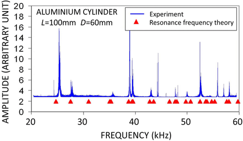
Figure 19 compares the experimental resonance curve (in solid blue line) with the theoretical resonance frequencies (in red triangles) computed from the elastic velocities independently measured by pulse transmission (PT). As far as the excited resonance modes are concerned, the agreement between experiment and theory is fairly good. Furthermore, this is consistent with the fact that the elastic velocities inverted from the resonance curves (i.e., V_P = 6495 m/s and V_S = 3111 m/s) are quite close to the elastic velocities independently measured by PT (i.e., V_P = 6469 m/s and V_S = 3104 m/s). The deviations are as small as 0.4% on V_P and 0.2% on V_S.

5.2 Results in Plexiglas

Now we test the procedure with a homogeneous but absorbing material, namely Plexiglas.

Figure 20 is similar to the previous one, with the same plot convention but corresponds to a Plexiglas cylinder of the same dimension.

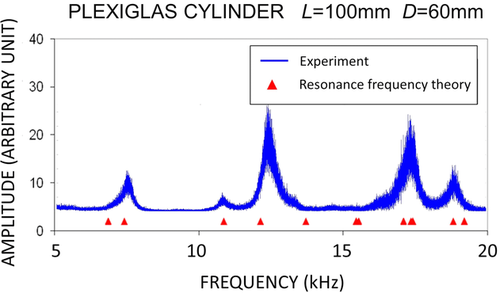
The agreement between experiment and theory is not as good as in the case of the aluminium cylinder but is still acceptable. More precisely, the inverted P-wave and S-wave velocities (i.e., V_P = 2685 m/s and V_S = 1376 m/s) from the resonance curves are rather close to the elastic velocities independently measured by PT (i.e., V_P = 2700 m/s and V_S = 1370 m/s), with deviations as small as 0.6% on V_P and 0.5% on V_S.

The accurate velocity measurements in the attenuating Plexiglas achieved by our methodology based on noise correlation is an additional confirmation of correct velocity measurements in dissipative media using seismic interferometry, as reported by Roux et al. (2005) and Slob and Wapenaar (2007), and reminded by Wapenaar et al. (2010b).

Further information can be extracted about attenuation from the resonance curve plotted in Fig. 20. Focusing on one of the resonance peaks, for instance, the one around 12.3 kHz, the quality factor corresponding to this resonance mode deduced from the relative peak width at half power is Q ≈ 28 (see Bourbié et al. 1987 or Lucet 1989), which is consistent with the quality factors obtained by Lucet (1989) using resonant bars for frequencies around a few kilohertz, namely Q_E ≈ 29–35 for extensional (E) mode and Q_T ≈ 25–27 for torsional (T) or shear mode.

5.3 Results in Vilhonneur limestone

Vilhonneur limestone is a well-cemented and weakly permeable (permeability k ≈ 0.3 mD) oolitic limestone, exhibiting abundant microporosity in the oolites (porosity φ ≈ 11%) (e.g., Lucet 1989).

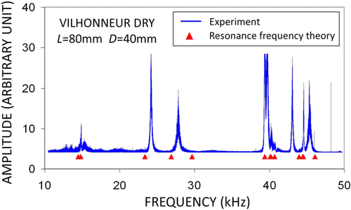
Figure 21 shows the results on a cylinder sample (diameter D = 4 cm and length L = 8 cm) of dry Vilhonneur limestone, with the same plot conventions as Fig. 19. The agreement between the experimental results and the theoretical prediction corresponding to the inverted model is not as good as for the case of aluminium but is still acceptable. More precisely, the elastic velocities inverted from ultrasonic interferometry (UI) (i.e., V_P = 4306 m/s and V_S = 2375 m/s) do not substantially differ from the velocities independently measured by PT (i.e., V_P = 4285 m/s and V_S = 2438 m/s), with 0.5% accuracy on V_P and 2.5% on V_S. As for aluminium, density of the rock sample (ρ = 2390 kg·m⁻³) was measured independently by weighing.

5.4 Limits of the method

This experimental procedure, involving the principles of both passive seismic interferometry and resonance ultrasound spectroscopy (RUS), is validated at ambient conditions. Achieving RUS experiments under higher pressures and temperatures is not an issue (see for instance Lucet et al. 1991; Isaac et al. 1998). Nevertheless, the noise generation under such conditions (i.e., inside a pressure and temperature cell) is not as straightforward as at ambient conditions since the energy equipartition of the noise has to be respected in order to apply passive seismic interferometry.

Another limitation is the impact of the attenuation. Strictly speaking, the RUS-inverse code cannot deal with attenuation and assumes that the considered sample is lossless. Thus, when dealing with attenuating samples, before running the RUS-inverse code itself, Zadler et al. (2004) recommend to fit point by point each resonance peak composing the resonance curve with theoretical Lorentzian resonance curve. In practice, it is difficult to run this procedure with too attenuating media, such as a water-saturated rock. In many cases, the resonance curve is then so noisy that it is tricky to achieve a resonance curve fitting point by point. Overcoming this kind of issues is beyond the scope of this paper and will be described in a further companion paper.

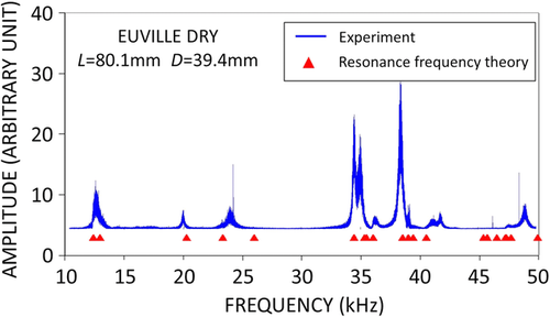
Moreover, the inversion procedure cannot deal with strongly heterogeneous media. For instance, Fig. 22 shows the resonance spectrum of a sample of Euville limestone, which is known as a heterogeneous rock (e.g., Lucet 1989). Even if the resonance peaks are clearly identifiable, the inversion code does not give very good results. The deviations are as large as 8.8% on V_S (i.e., V_S = 2278 m/s by UI and V_S = 2077 m/s by PT) and 2.5% on V_P (i.e., V_P = 3670 m/s by UI and V_P = 3766 m/s by PT). This is simply explained by the fact that the inversion code is running outside its range of validity when dealing with heterogeneous media, as already pointed out by Zadler et al. (2004).