3-D shallow-water seismic survey evaluation and design using the focal-beam method: a case study offshore Abu Dhabi
ABSTRACT
For 3-D shallow-water seismic surveys offshore Abu Dhabi, imaging the target reflectors requires high resolution. Characterization and monitoring of hydrocarbon reservoirs by seismic amplitude-versus-offset techniques demands high pre-stack amplitude fidelity. In this region, however, it still was not clear how the survey parameters should be chosen to satisfy the required data quality. To answer this question, we applied the focal-beam method to survey evaluation and design. This subsurface- and target-oriented approach enables quantitative analysis of attributes such as the best achievable resolution and pre-stack amplitude fidelity at a fixed grid point in the subsurface for a given acquisition geometry at the surface. This method offers an efficient way to optimize the acquisition geometry for maximum resolution and minimum amplitude-versus-offset imprint. We applied it to several acquisition geometries in order to understand the effects of survey parameters such as the four spatial sampling intervals and apertures of the template geometry. The results led to a good understanding of the relationship between the survey parameters and the resulting data quality and identification of the survey parameters for reflection imaging and amplitude-versus-offset applications.
INTRODUCTION
Seismic survey parameters should be chosen such that the acquired data have the quality required to achieve the objectives in exploration, appraisal, and development of oil and gas fields. Several authors have presented sophisticated approaches to survey evaluation and design in order to obtain a high data quality while mitigating the survey effort. Traditionally, survey design is based on bin attributes such as fold, offset, and azimuth sampling in each bin, as well as their distribution across bins. Such aspects are discussed by Cordsen, Galbraith, and Peirce (2000); Galbraith (2004); and Vermeer (2012). In this approach, the information is obtained from a given acquisition geometry at the surface, but subsurface structures and properties are not taken into account. Therefore, this approach may be valid for a nearly homogeneous subsurface, but it is no longer adequate for a complex subsurface. Recently, survey design has started to involve full simulation of a seismic experiment for a given acquisition geometry, full processing of the simulated seismic data to evaluate the resulting image quality, and full inversion of the processed data to evaluate the resulting quality of the estimated reservoir properties. However, these results include the combined effects of the acquisition geometry, processing, and inversion and, therefore, obscure the effects purely due to the given acquisition geometry. In addition, this approach is computationally expensive, making it impractical if acquisition geometries need be designed over and over again. A more efficient approach to survey design involves the reconstruction of the angle-dependent reflectivity in one or more subsurface points in the target area. The input data consist in the waves scattered from a single subsurface point for a given acquisition geometry and an assumed subsurface model. After wave-equation-based pre-stack depth migration, the imaging quality of the reconstructed angle-dependent reflectivity in the subsurface point is then used to evaluate the acquisition geometry. This reflectivity is equivalent to the Hessian for angle-dependent least squares wave-equation-based pre-stack depth migration (e.g., Ren, Wu, and Wang (2011)) but evaluated for a subsurface point that does not introduce any angle dependence. An example is the focal-beam method, which was initially developed by Berkhout et al. (2001) and Volker et al. (2001) and further expanded by van Veldhuizen, Blacquière, and Berkhout (2008) and Wei, Fu, and Blacquière (2012). This method makes use of the common focus point technology (Berkhout 1997a,b), in which the seismic response is decomposed into individual subsurface points, and the migration response is modelled for one or more specific subsurface points and for a given acquisition geometry. Therefore, this method can be applied to survey evaluation and design as a subsurface- and target-oriented approach to obtain certain attributes for one or more subsurface points rather than for the whole subsurface volume.
In a shallow-water environment like the Gulf region in the Middle East, 3-D ocean bottom cable (OBC) and ocean bottom node (OBN) seismic surveys are often acquired under operational constraints such as shallow-water depths and numerous production facilities distributed in a scattered way over the survey area. In these seismic surveys, receivers and sources are independently deployed. Therefore, the survey design is highly flexible, allowing for a variety of acquisition geometries. Ishiyama, Painter, and Belaid (2010c); Ishiyama, Mercado, and Belaid (2012); and Nakayama, Belaid, and Ishiyama (2013) describe the comprehensive properties of and several options for a shallow-water acquisition geometry. The relevant survey parameters are the four spatial sampling intervals and apertures of the template geometry, similar to those of marine and land seismic surveys (Vermeer 2012). The four spatial sampling intervals are defined by the receiver and source intervals, each in two sampling directions that are usually orthogonal. The four spatial sampling apertures consist in the receiver and source apertures, oriented in the same way as the above four spatial coordinates. Proper spatial sampling can be viewed as the ability to properly reconstruct seismic wavefields. Wide apertures, i.e., a large extent of the template geometry, enhance the ability to reconstruct seismic wavefields in terms of spatial continuity. In addition, this is beneficial for fault imaging and fracture characterization in the region (e.g., Ishiyama et al. (2010b)).
- (i) What is the relationship between the survey parameters and the resulting data quality?
- (ii) Which types of survey parameters are essential?
In this paper, we adopted the focal-beam method to try to answer these questions. This subsurface- and target-oriented approach enables quantitative analysis of the achievable resolution and pre-stack amplitude fidelity for one or more grid points in the subsurface and for a given acquisition geometry at the surface. We start with an overview of the focal-beam method, apply it to 3-D shallow-water seismic survey evaluation and design offshore Abu Dhabi, and end with a discussion on the relationship between the survey parameters and the resulting data quality.
FOCAL-BEAM METHOD
First, we discuss the survey parameters and define survey effort. Then, we summarize the focal-beam method. In this method, migration is described as a double-focusing process to 3-D seismic data. The output is presented as the combined result of focal beams, namely, focal detector beam and focal source beam, revealing the migration response by focal functions, i.e., the resolution by resolution function and the pre-stack amplitude fidelity by AVP function. For further theoretical and mathematical details, we refer the reader to the papers by Berkhout et al. (2001), Volker et al. (2001), van Veldhuizen et al. (2008), and Wei et al. (2012). We will adopt the mathematical notation of these authors: matrices are bold with upper case; vectors are in italics with a right arrow symbol  . In addition, we will sometimes use the word “detector” for “receiver”.
Survey parameters and survey effort
As aforementioned, for 3-D shallow-water seismic surveys, the relevant survey parameters are the spatial sampling intervals for receivers  and
and  and for sources
  and
and  as well as their respective apertures,
  and
and  for the receivers and
  and
and  for the sources in the template geometry. For an orthogonal geometry, the basic subset is a cross-spread gather, where receiver-point and source-point intervals are quite fine (
 and
and  for example), whereas receiver-line and source-line intervals are often coarse (
 and
and  in this example). Receiver-line and source-line lengths specify the maximum apertures (
 and
and  for this basic subset). For an areal geometry, the basic subset is a common-receiver gather, where receivers are arranged on a sparsely spaced grid (
 and
and  ), whereas sources are on a densely spaced grid (
 and
and  ). Source-spread widths (
 and
and  ) specify the maximum apertures. This is because deployment of receivers usually requires more effort than that of sources in shallow-water seismic surveys. It should be noted that, from these survey parameters, traditional survey attributes such as bin size, nominal fold, trace density, maximum offset, and largest minimum offset can be directly calculated.
 , specify the spatial sampling of the basic subset, where subscript b can be either d or s, independently for each survey parameter but not in arbitrary combinations. Two other coordinates, the set
  , specify the spatial redundancy of the basic subsets, i.e., the fold, where again subscript B can be d or s. Their maximum apertures,
  and
and  , are usually the same as
  and
and  to form the template. For instance, the set
  specifies the spatial sampling of a cross-spread gather, i.e.,
  , whereas the set
  specifies the spatial redundancy of the cross-spread gather, i.e.,
  . For another example, the set
  specifies the spatial sampling of a common-receiver gather, whereas the set
  specifies the spatial redundancy of the common-receiver gather, i.e.,
 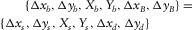 . Here, the x-direction is considered as the in-line direction. The survey effort C can be defined as a combined attribute of these survey parameters relative to a reference template
 (1)
(1) is the survey effort for each component,
  ,
,  ,
,  ,
,  , and
, and  . Subscript “ref” denotes “reference”; factors
  and
and  are the template-repeat factors resulting from rolling the template in the in-line and the cross-line directions while repeating a part of the template. The attributes in terms of symmetry can be also defined as
 (2)
(2) (3)
(3) (4)
(4) and
and  are the aspect ratios of the spatial sampling intervals, and
  is the aspect ratio of the spatial sampling apertures. For instance, if a reference template consists of
 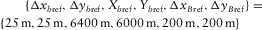 with
with  and
and  , for a template consisting of
 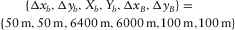 with
with  and
and  , then
  ,
,  ,
,  ,
,  ,
,  ,
,  ,
,  , and
, and  . See, for example, Table 1. These survey parameters and attributes express the specification of seismic data.
| Geometry |  (m) (m) |
 (m) (m) |
 (m) (m) |
 (m) (m) |
 (m) (m) |
 (m) (m) |
 |
 |
C |
|---|---|---|---|---|---|---|---|---|---|
| OR1144 | 12.5 | 12.5 | 400 | 400 | 6400 | 6000 | 1 | 1 | 1.00 |
| OR2222 | 25.0 | 25.0 | 200 | 200 | 6400 | 6000 | 1 | 1 | 1.00 |
| OR4411 | 50.0 | 50.0 | 100 | 100 | 6400 | 6000 | 1 | 1 | 1.00 |
| OR4122 | 50.0 | 12.5 | 200 | 200 | 6400 | 6000 | 1 | 1 | 1.00 |
| OR2241 | 25.0 | 25.0 | 400 | 100 | 6400 | 6000 | 1 | 1 | 1.00 |
| AR284Q | 25.0 | 100.0 | 400 | 25 | 6400 | 6000 | 1 | 1 | 1.00 |
| AR244H | 25.0 | 50.0 | 400 | 50 | 6400 | 6000 | 1 | 1 | 1.00 |
| AR2241 | 25.0 | 25.0 | 400 | 100 | 6400 | 6000 | 1 | 1 | 1.00 |
| OR2222_10R5 | 25.0 | 25.0 | 200 | 200 | 6400 | 3000 | 1 | 2 | 1.00 |
| OR2222_10R5_SLI | 25.0 | 25.0 | 200 | 400 | 6400 | 6000 | 1 | 2 | 1.00 |
| Geometry |  (m) (m) |
 (m) (m) |
 (m) (m) |
 (m) (m) |
 |
 |
 |
 |
 |
| OR1144 | 12.5 | 12.5 | 6400 | 6000 | 1.00 | 0.94 | 2.00 | 2.00 | 4.00 |
| OR2222 | 25.0 | 25.0 | 6400 | 6000 | 1.00 | 0.94 | 1.00 | 1.00 | 1.00 |
| OR4411 | 50.0 | 50.0 | 6400 | 6000 | 1.00 | 0.94 | 0.50 | 0.50 | 0.25 |
| OR4122 | 50.0 | 12.5 | 6400 | 6000 | 4.00 | 0.94 | 0.50 | 2.00 | 1.00 |
| OR2241 | 25.0 | 25.0 | 6400 | 6000 | 1.00 | 0.94 | 1.00 | 1.00 | 1.00 |
| AR284Q | 25.0 | 100.0 | 6400 | 6000 | 0.25 | 0.94 | 1.00 | 0.25 | 0.25 |
| AR244H | 50.0 | 50.0 | 6400 | 6000 | 1.00 | 0.94 | 0.50 | 0.50 | 0.25 |
| AR2241 | 100.0 | 25.0 | 6400 | 6000 | 4.00 | 0.94 | 0.25 | 1.00 | 0.25 |
| OR2222_10R5 | 25.0 | 25.0 | 6400 | 3000 | 1.00 | 0.47 | 1.00 | 0.50 | 0.50 |
| OR2222_10R5_SLI | 25.0 | 25.0 | 6400 | 6000 | 1.00 | 0.94 | 1.00 | 1.00 | 1.00 |
| Geometry |  (m) (m) |
 (m) (m) |
 (m) (m) |
 (m) (m) |
 |
 |
 |
 |
 |
| OR1144 | 400 | 400 | 6400 | 6000 | 1.00 | 0.94 | 0.50 | 0.50 | 0.25 |
| OR2222 | 200 | 200 | 6400 | 6000 | 1.00 | 0.94 | 1.00 | 1.00 | 1.00 |
| OR4411 | 100 | 100 | 6400 | 6000 | 1.00 | 0.94 | 2.00 | 2.00 | 4.00 |
| OR4122 | 200 | 200 | 6400 | 6000 | 1.00 | 0.94 | 1.00 | 1.00 | 1.00 |
| OR2241 | 400 | 100 | 6400 | 6000 | 4.00 | 0.94 | 0.50 | 2.00 | 1.00 |
| AR284Q | 25 | 400 | 6400 | 6000 | 0.06 | 0.94 | 8.00 | 0.50 | 4.00 |
| AR244H | 25 | 400 | 6400 | 6000 | 0.06 | 0.94 | 8.00 | 0.50 | 4.00 |
| AR2241 | 25 | 400 | 6400 | 6000 | 0.06 | 0.94 | 8.00 | 0.50 | 4.00 |
| OR2222_10R5 | 200 | 200 | 6400 | 3000 | 1.00 | 0.47 | 1.00 | 2.00 | 2.00 |
| OR2222_10R5_SLI | 200 | 400 | 6400 | 6000 | 0.50 | 0.94 | 1.00 | 1.00 | 1.00 |
Forward model
 -f) domain. Each matrix multiplication represents a multi-dimensional spatial convolution. Each element of every matrix contains amplitude and phase information. In this model, seismic data can be described for each monochromatic component as
 (5)
(5) is the data matrix of the primary wavefields recorded by detectors at depth
  due to sources at depth
  , both depths being close to zero (Fig. 1). A row and a column of the data matrix correspond to a certain detector location d at
  and a certain source location s at
  , respectively. For regular spatial sampling,
  ,
,  ,
,  , and
, and  ; see, for example, Fig. 1(a) and (b). Furthermore,
  ,
,  ,
,  , and
, and  , where max( · ) and min( · ) are the maximum and the minimum values for each component. According to the row and column numbering, a row
  constitutes a common-receiver gather, a column
  constitutes a common-source gather, and a submatrix specified by rows for receivers of a receiver line and columns for sources of a source line represents a cross-spread gather. The dagger symbol † is used to denote a row vector. Common-offset gathers and common-midpoint gathers are identified in the data matrix as diagonals and anti-diagonals, respectively. An element
  constitutes one frequency component of a single trace recorded by the
  detector and shot by the
  source, i.e.,
  .
. is the reflectivity matrix representing the conversion of the incident wavefields into the reflected wavefields at depth
  (Fig. 2). In the same manner as the data matrix, a row and a column of the reflectivity matrix correspond to a certain grid-point location i at
  and a certain grid-point location j at
  , respectively. Subscripts i and j indicate variable locations while, later on, subscript k will be used for a particular location. An element
  represents one frequency component of a reflected wavefield at the
  grid point generated by a delta function source at the
  grid point, i.e.,
  .
. is the source matrix, its columns
  containing the source properties at
  , i.e.,
  .
. is the propagation matrix, its columns containing the downgoing wavefields at
  generated by delta function sources at
  . An element of the downgoing wavefields
  represents a direct wavefield at
  caused by a delta function source at
  , i.e.,
  .
. is the propagation matrix, its columns containing the upgoing wavefields at
  generated by delta function sources at
  . An element of the upgoing wavefields
  represents a direct wavefield at
  caused by a delta function source at
  , i.e.,
  .
. is the detector matrix, its rows
  containing the detector properties at
  , i.e.,
  .
.

 for a certain source s at
  with all frequencies (a) in the 2-D d-t domain and (b) in the 3-D
  -t domain. A common-receiver gather
  can be considered in the same way but for a certain detector d at
  . Seismic data
  with all frequencies (c) in the 3-D
  -t domain and (d) in the 3-D
  -ω domain are described by (e) and (f) data matrix
  for each monochromatic component.
 for each monochromatic component.
Later on, the spatial coordinate z will sometimes be omitted for brevity. In the case that W represents one-way wave propagation, equation 5 can be viewed as the Born approximation to the Lippmann–Schwinger equation with a one-way Green's function W. Equation 5 is a general description of seismic data. In the case of blended acquisition with the blending operator  ,
,  can replace S in this equation (Berkhout 2008). For a full-wavefield model that includes not only the primary wavefields but also the secondary wavefields generated by surface-related and internal multiples, a full-wavefield propagator or Green's function G can replace W in this equation (Kumar, Blacquière, and Verschuur (2014)). Note that, with all frequencies, the matrices in the frequency domain can be envisaged more naturally in the time domain. Since the discrete Fourier transform is invertible, either domain can be used depending on the application. Also note that this forward model is valid for stationary or parts of non-stationary acquisition geometries.
Double focusing
 , and subsequently removing the effects of wave propagation in the overburden, i.e., going from
  to R. Therefore, migration aims at removing
  at the detector side and
  at the source side for the selected grid point. In the WRW model for a particular depth
  only, double focusing can be described as
 (6)
(6) is the grid-point matrix or estimated reflectivity matrix at
  (Fig. 2). The hat symbol
  is used to denote “estimated”.
  is an element of the grid-point matrix.
 and
and  are the one-way focusing operators removing the wave propagation in the overburden above
  , or in other words, focusing at
  from the surface.
  focuses at the
  grid point at the detector side, and
  focuses at the
  grid point at the source side.
A perfect migration requires  and
and  , where
  is the identity matrix. In this perfect case,
  is equal to
  . From this concept, survey design can be thought of as choosing S and D to obtain a satisfactory migration response, i.e., to obtain a good estimate of
  .
.
There are two approaches in the double focusing, i.e., confocal imaging and bifocal imaging. Confocal imaging results in a scalar image of angle-averaged reflectivity by assuming that a certain grid-point location to be focused at the detector side is the same as that at the source side. In this case, i is identical to j at a particular location k, i.e.,  in equation 6 and Fig. 2, and the angle-averaged reflectivity
  at the
  grid point is obtained. Alternatively, bifocal or extended imaging yields a vector image of angle-dependent reflectivity by considering that grid-point locations to be focused at the source side are around a certain grid-point location to be focused at the detector side, or vice versa. In this case, j varies around a particular location k, or vice versa, i.e.,
  and j varying around k or
  and i varying around k in equation 6 and Fig. 2, and the angle-dependent reflectivity
  or
or  at the
  grid point is obtained. This result respects angle-dependent reflectivity information between the incident wavefields and the reflected wavefields. In other words, a plane-wave decomposition of such a result by a linear Radon transform reveals the AVP response (de Bruin, Wapenaar, and Berkhout 1990). Therefore, once the angle-dependent reflectivity is obtained by bifocal imaging, the AVP response can be obtained by transforming the results to the Radon domain (e.g., Verschuur and Berkhout (2011)). This is in contrast with conventional AVP techniques in which the AVP response is obtained by tracking the amplitude change along the reflection in a pre-stack domain. Furthermore, obtaining
  for all frequencies and applying the imaging principle, i.e., imaging at zero time and at zero intercept time, produces results in the spatial (
 ) domain and in the Radon (
 ) domain, respectively. Note that this idea forms the basis of angle-dependent reflectivity retrieval (MacKay and Abma 1992; Rickett and Sava 2002; Biondi and Symes 2004; Duveneck 2013) and velocity analysis (Shen and Symes 2008; Symes 2008; Mulder 2008, 2014) by means of extended images.
Grid-point decomposition
 (7)
(7) (8)
(8) contains only the response of the
  grid point, and
  is obtained with
  by equation 5. Symbol δ is used to emphasize one grid-point diffractor.
For an angle-independent unit-point diffractor at the  grid point,
  contains only one non-zero element, i.e.,
  for
for  and
and  for
for  or
or  , representing the total reflection of the incident wavefield into the reflected wavefield only at the
  grid point.
Focal beams
The focal detector beam is introduced as  at the detector side, and the focal source beam is introduced as
  at the source side in equation 6. Considering a unit-point diffractor
  at the
  grid point, i.e.,
  in equation 6, the focal beams contain angle-dependent sensing and illumination information that is introduced by the acquisition geometry at the surface since the reflectivity at the
  grid point in the subsurface has been set to be angle independent. In other words, a plane-wave decomposition of the focal beams by a linear Radon transform reveals angle-dependent sensing and illumination imprints caused by the source geometry and the detector geometry.
 only (Fig. 3(b) and (c)) can be described as
 (9)
(9) focused at the
  grid point. Consequently, the focal detector beam contains information predominantly from the detector geometry.
 only (Fig. 3(e) and (f)) can be described as
 (10)
(10) focused at the
  grid point. As a consequence, the focal source beam contains information predominantly from the source geometry.
Ideally, the focal beams should show a perfect unit-point sensing and illumination (Fig. 4(a)), i.e.,  and
and  . In the high-frequency approximation with infinite and dense detector and source coverage, this was proven by Beylkin and Burridge (1990) and ten Kroode, Smit, and Verdel (1998) and for extended images by ten Kroode (2012). However, this is not the case in practice because of acquisition geometry constraints given by the limited spatial sampling, the limited aperture, and the finite bandwidth of the seismic data. Similarly, the Radon-transformed focal beams should have amplitude spectra uniformly and evenly distributed over all angles (Fig. 4(b)). However, this is not the case in practice, again due to acquisition geometry constraints.

In summary, the focal detector beam reveals the sensing capability of the detector geometry and the focal source beam reveals the illumination capability of the source geometry in terms of spatial resolution in the space domain and pre-stack amplitude fidelity in the Radon domain. These properties offer the opportunity to separately evaluate the detector geometry and the source geometry.
Focal functions
The resolution function (Fig. 3(h)) is introduced as a confocal imaging result for a unit-point diffractor  at the
  grid point, i.e.,
  in equation 6. The resolution function is defined as the diagonal of the resulting grid-point matrix after double-focusing, i.e.,
  varying around k. The right-hand side of this equation is equivalent to
  . Recall a unit-point response, i.e.,
  for
for  , and
, and  for
for  or
or  . In this case, for a stationary acquisition geometry, the resolution function can be efficiently obtained by an element-by-element multiplication of the focal detector beam
  and the focal source beam
  , i.e., the product rule in the space domain (Berkhout et al. 2001; van Veldhuizen et al. 2008). Ideally, the resolution function should correspond to a perfect unit-point response in a similar fashion as the focal beams (Fig. 4(a)), i.e.,
  for
for  and
and  for
for  or
or  . However, this hardly occurs in practice due to acquisition geometry constraints. Fortunately, because of the product rule, deficiencies in the focal detector beam are often compensated for by the focal source beam, or vice versa, possibly resulting in a satisfactory resolution function.
The AVP function (Fig. 3(i)) is introduced as a bifocal imaging result for an angle-independent unit reflector  , including the
  grid point, i.e.,
  in equation 6. Symbol Δ is used to denote one single reflector. The right-hand side of this equation is equivalent to
  . Notice a unit-reflector response, i.e.,
  . In this case, for a stationary acquisition geometry, the AVP function can be approximated by a convolution of the focal detector beam
  and the focal source beam
  and, therefore, by an element-by-element multiplication of the Radon-transformed focal detector beam and the Radon-transformed focal source beam, i.e., the product rule in the Radon domain as defined by Berkhout et al. (2001) and mathematically proven by van Veldhuizen et al. (2008). Ideally, the AVP function should have amplitude spectra uniformly and evenly distributed over all angles in a similar fashion as the Radon-transformed focal beams (Fig. 4(b)). However, this seldom occurs in practice, again due to acquisition geometry constraints. In this case, the AVP function reveals the angle-dependent imprint caused by both the source geometry and the detector geometry.
In summary, the resolution function reveals the achievable spatial resolution in the space domain, and the AVP function shows the achievable pre-stack amplitude fidelity in the Radon domain, both for the total acquisition geometry, i.e., the combination of the detector geometry and the source geometry. These properties offer the opportunity to optimize the acquisition geometry in order to efficiently maximize the spatial resolution and to effectively minimize the AVP imprint.
Survey evaluation and design using the focal-beam method
The focal-beam method enables survey evaluation and design. In this approach, the input information comprises an acquisition geometry at the surface, a subsurface model with the macro-velocities including one or more target grid points in the subsurface, and a focusing operator. With this information, the focal beams and the focal functions can be computed. For a non-stationary acquisition geometry, for example, with rolls in in-line and cross-line directions, the partial focal beams and the partial focal functions are computed for each stationary part. Then, the total focal beams and the total focal functions are obtained by summation of the partial ones (Fig. 3(k) and (l)). Note that the focal-beam method is most efficient for an acquisition geometry with large stationary parts such as 3-D OBC/OBN seismic surveys. With the focal beams and the focal functions, certain attributes can be quantitatively analysed, for instance, the achievable resolution and pre-stack amplitude fidelity, particularly the strength and width of the focusing result in the space domain and the spectral bandwidth and flatness of the focusing result in the Radon domain. In this way, the given acquisition geometry can then be evaluated against the required data quality for imaging and AVP applications of the target reflectors.
A CASE STUDY OFFSHORE ABU DHABI
We applied the focal-beam method to several acquisition geometries (Table 1) for 3-D shallow-water seismic survey evaluation and design offshore Abu Dhabi. The abbreviation “OR” stands for “orthogonal”, and “AR” stands for for “areal”. In the region, earlier studies suggested two attributes required to image the target reflectors (Ishiyama et al. 2010c): a trace density, i.e., nominal fold per bin size, of about 1.5 /m2, and a maximum offset, i.e., half of a maximum aperture, of about 3800 m corresponding to a maximum inline offset of about 3200 m with the 85 % rule (Cordsen et al. 2000). The acquisition geometries in Table 1 satisfy these criteria. Notice that, in all cases, the trace density and the survey effort are equally constant, i.e.,  /m2 and
  . For the subsurface model, the layered P-wave and S-wave velocity models were built from well log data in the region. The target grid point was set at a depth level of the Upper Jurassic formations and at the center of a horizontal area of 8 km × 8 km. The average P-wave velocity around the target level is about 4 km/s, the interval P-wave velocity about 6 km/s, and the interval S-wave velocity about 3.2 km/s. For the wave propagation operator, recursive and explicit one-way extrapolation operators (e.g., Blacquière et al. (1989); Thorbecke, Wapenaar, and Swinnen (2004)) were used both for the forward modelling and for the double focusing. The focal beams and the focal functions were computed up to a maximum frequency of 50 Hz.
Effects of spatial sampling intervals with the symmetry
Figure 5 shows the results from three acquisition geometries: OR1144, OR2222, and OR4411 in Table 1, which have the same spatial sampling apertures but different intervals. These are orthogonal geometries in which the receiver lines are deployed in the x-direction, whereas the source lines are oriented in the y-direction. These acquisition geometries almost meet the symmetric sampling criterion: the receiver-point interval is equal to the source-point interval,  and
and  ; the receiver-line interval is identical to the source-line interval,
  and
and  ; the receiver-line length is almost the same as the source-line length,
  and
and  . Figure 5(a) shows the acquisition geometry spreads, where blue triangles and red circles indicate receivers and sources, respectively.

Figure 5(b) and (c) shows the focal detector beams in the space domain and in the Radon domain, respectively. In the space domain, the axes are the x- and y-distances from the target grid point. In the Radon domain, the axes indicate the ray parameters  and
and  related to the target grid point. The maximum of the axes is the slowness at the target grid point, i.e., the inverse of the interval velocity with an angle of 90°. The colour scale represents the normalized amplitude. In the space domain, a well-focused lobe is found at the target grid point for all three cases because of adequate spatial sampling apertures. However, some aliasing effects are present in the y-direction for OR1144 and OR2222 due to the coarse spatial sampling interval in this direction. In the Radon domain, a broad range of angles is seen for all three cases because of the high aspect ratio of the apertures. However, some band-like features exist with a periodicity in the y-direction for OR1144 and OR2222 due to aliasing effects. OR4411 shows no obvious deficiency because of the relatively fine sampling in both the x- and y-directions. Figure 5(d) and (e) shows the focal source beams. The same observations can be made but in the other direction, i.e., in the x-direction in this case.
Figure 5(f) and (g) shows the resolution functions and the AVP functions, respectively. For the resolution function, a well-focused lobe is found only at the target grid point and no aliasing effect is observed away from it for all three cases. This is because aliasing effects occur in two orthogonal directions, i.e., in the y-direction for the focal detector beam and in the x-direction for the focal source beam. These effects are cancelled by the product rule for the resolution function. Because of the product rule, the deficiencies in the focal detector beam are compensated for by the focal source beam, or vice versa, and this results in the satisfactory resolution function. This explains why most common acquisition geometries achieve a quite acceptable resolution. In fact, this agrees with the suggestion of Vermeer (2010) that proper spatial sampling for imaging implies proper sampling of two of the four spatial coordinates. The results show that the resolution function is robust against the aliasing effects and that the resolution is not much affected by the acquisition geometry if the detector geometry and the source geometry have different coarse sampling directions and if their apertures are adequate. This means that the spatial sampling intervals and apertures of the basic subset,  ,
,  ,
,  , and
, and  , are the essential types of survey parameters for reflection imaging. For the AVP function, AVP imprints related to the acquisition geometry are clearly seen for OR1144 and OR2222. This is because the aliasing effects expanded over angles, both for the focal detector beam and the focal source beam, are intensified by the product rule for the AVP function. This is not the case for OR4411 because of no obvious deficiency in either the focal detector beam or the focal source beam. These results show that the AVP imprints are sensitive to the aliasing effects and that the pre-stack amplitude fidelity is easily affected by the acquisition geometry. To obtain the ideal AVP function, proper sampling of all four spatial coordinates may be required, although this condition is obviously demanding. This means that all the four spatial sampling intervals and apertures of the template geometry,
  ,
,  ,
,  ,
,  ,
,  , and
, and  , are essential for AVP applications.
Effects of spatial sampling intervals with the asymmetry
We now compare the results from six acquisition geometries: OR4122, OR2222, OR2241, AR284Q, AR244H, and AR2241 in Table 1, which have the same spatial sampling apertures, but again different intervals. OR4122 has a receiver-point interval differing from the source-point interval, OR2241 has a receiver-line interval differing from the source-line interval, and therefore, they are asymmetric. AR284Q, AR244H, and AR2241 are areal geometries to be acquired with parallel swath shooting in which the receiver lines and the source lines are parallel in the x-direction. The receivers are arranged sparsely in the y-direction while the sources are on a densely spaced grid, and therefore, these are asymmetric. From the four spatial coordinates' point of view, OR2241 and AR2241 are equivalent.
The results in Fig. 6 exhibit the acquisition geometry spreads and the focal functions. For the resolution function, a well-focused lobe is found only at the target grid point and no aliasing effect is observed away from it for all six cases. These results again show the robustness of the resolution function, regardless of the asymmetry. For the AVP function, OR4122 and OR2222 show subtle AVP imprints. However, others display severe band-like features with a periodicity in the coarse sampling direction, i.e., in the y-direction in this case. These results show that the AVP spectral flatness depends on the sparsity of the acquisition geometry and is severely affected in the coarse sampling direction, regardless of the asymmetry and the acquisition geometry type.

Effects of spatial sampling apertures and the symmetry
Figure 7 shows the results of OR2222 in Table 1. Now, we consider three cases with different spatial sampling apertures, roll patterns, and resulting aspect ratios of the apertures, i.e., OR2222, OR2222_10R5, and OR2222_10R5_SLI. Generic choices for the OBC/OBN acquisition geometry are made: a 10-roll-5-receiver-line roll whereby 10 receiver lines are active in the current patch while 5 extra receiver lines are rolled from the previous patch to the following patch in the cross-line direction during the shooting in the current patch, i.e., a source-line interleave whereby source lines in a patch are interleaved by source lines from the previous and following patches (Ishiyama et al. 2012). OR2222_10R5 adopts 10-roll-5-receiver-line roll, a patch of which has a cross-line aperture and an aspect ratio of half those of OR2222. OR2222_10R5_SLI corresponds to OR2222_10R5 with the source-line interleave, a patch of which has the same crossline aperture and aspect ratio as those of OR2222. Both of them cover the whole surface area by five rolls in this case.

The results in Fig. 7 exhibit the patch spreads of the acquisition geometries and the focal functions. For the resolution function, the same observations can be made in all three cases. For the AVP function, OR2222 and OR2222_10R5_SLI show a broad expanse, although OR2222_10R5_SLI has reasonable but no extra dilation in the cross-line direction. Besides, OR2222_10R5 displays a limited bandwidth in the cross-line direction, i.e., in the y-direction in this case. These results show that the AVP spectral bandwidth depends on the spatial sampling aperture in the cross-line direction and the resulting aspect ratio of the apertures and is constrained by the shorter aperture in the crossline direction, regardless of the acquisition geometry type and roll pattern.
Effects of wave types to be recorded
Figure 8 shows the results of OR2222 in Table 1. Now, the three cases have different wave types to be recorded: OR2222, OR2222_PS, and OR2222_SS. Using converted waves is a natural and interesting option since one of the advantages of OBC/OBN seismic surveys is a direct S-wave measurement by a 4-C receiver, although these waves have not yet been fully utilized in the region today. For the P-S wave, the conversion from P-wave to S-wave is assumed to occur at the target grid point during the reflection. The focal source beam is computed with the P-wave velocity model, the focal detector beam is computed with the S-wave velocity model, and these focal beams are straightforwardly combined to obtain the focal functions. For the (P-)S-S wave, a conversion from P-wave to S-wave is supposed to occur near the surface. In the region, a dominant mode conversion to S-wave near the surface exists because of the very shallow-water depth and the hard sea bottom. These events are confirmed in existing seismic data recorded by horizontal-component geophones (Berteussen and Sun 2010). In this case, both the focal beams and the focal functions are computed with the S-wave velocity model.

The results in Fig. 8 exhibit the focal beams and the focal functions. For the focal beams, the same observations can be made as in the previous examples except for the range of ray parameters for S-waves. The maximum ray parameter for an S-wave is much larger than that for a P-wave because of the lower interval velocity at the target grid point. The maximum ray parameter in the axes for a P-wave corresponds to 90° in angle and is comparable with about 30° for an S-wave, and therefore, wider extents of ray parameters for the focal detector beam of OR2222_PS and for both the focal detector beam and the focal source beam of OR2222_SS are found. However, for OR2222_PS, the attainable extent is limited by the aperture of the source geometry. To fully acquire the extent of the ray parameter, a wider aperture of the source geometry would be required. For the resolution function, OR2222_PS and OR2222_SS show a sharper resolution because of the shorter S-wave length. However, for the AVP function, OR2222_PS and OR2222_SS display more severe AVP imprints due to the stronger aliasing effects caused by the lower S-wave velocity while keeping the spatial sampling intervals the same. These results show that the resolution function improves; however, AVP imprints become seemingly worse when utilizing the converted waves. To obtain the ideal AVP function, a much finer sampling of the four spatial coordinates would be required. However, AVP applications for seismic reservoir characterization using jointly P-waves and converted waves are more robust than those using only P-waves even for a limited range of ray parameter and more severe AVP imprints (van Veldhuizen et al. 2008). Therefore, much finer sampling may not always be required for utilizing converted waves.
DISCUSSION
- Resolution is robust and not much affected by the aliasing effects introduced by the acquisition geometry if it has two different fine-sampling directions while satisfying the required apertures. At least two of the four spatial coordinates should be sampled densely, and the other coordinates can be sampled in an affordable manner. This means that the spatial sampling intervals and apertures of the basic subset,
 ,
,  ,
,  , and
, and  , are essential for reflection imaging.
 - Pre-stack amplitude fidelity is sensitive to and easily affected by the aliasing effects. First, the AVP spectral flatness is severely affected in the coarse sampling direction, regardless of the symmetry, the asymmetry, and the acquisition geometry type. The sparsity should not be thrust into a particular sampling direction but should be shared by all four spatial coordinates. Second, the AVP spectral bandwidth is constrained by the shorter aperture in the cross-line direction, regardless of the acquisition geometry type and roll pattern. The aspect ratio should be close to one while satisfying the required apertures. This means that all the four spatial sampling intervals and apertures of the template geometry,
 ,
,  ,
,  ,
,  ,
,  , and
, and  , are essential for AVP applications.
 - Resolution improves, but pre-stack amplitude fidelity ostensibly deteriorates when utilizing converted waves while keeping the four spatial sampling the same, i.e., based on P-wave properties. However, the required pre-stack amplitude fidelity can be relaxed because of the robustness of seismic reservoir characterization using P-waves and converted waves jointly.
In this paper, we considered the capability of an acquisition geometry that enables imaging and AVP applications of target reflectors. However, in the region, seismic data are often dominated by surface waves masking the reflections. They impose additional requirements on the acquisition geometry since it should allow for effective surface-wave separation or removal (Berteussen, Zhang, and Sun 2011). We have recently discussed the essential types of survey parameters for surface-wave separation using signal-to-noise ratio (SNR) as an attribute representing the resulting data quality. We observed that the spatial sampling intervals of the basic subset,  and
and  , are essential in terms of surface-wave separation (Ishiyama, Blacquière, and Mulder 2014). Figure 9 illustrates which types of survey parameters are essential for surface-wave separation, reflection imaging, and AVP applications, respectively. Notice that parameters
  and
and  in the lower left of the figure are essential for surface-wave separation but also for reflection imaging and AVP applications. If these parameters are satisfactory for a required SNR given for the first, they usually also provide sufficient data quality for the others. This is because surface waves often correspond to a lower velocity than reflections and are more aliased.

Recently, the concept of random spatial sampling followed by data reconstruction has been introduced in survey design, which extracts broader spatial bandwidth from seismic data than that expected by the Nyquist criterion (e.g., Hennenfent and Herrmann 2008; Herrmann 2010). If reflection imaging and AVP applications are applied directly to the irregularly and under-sampled seismic data, an optimal acquisition geometry, for example, S and D with irregularly and sparsely distributed sources and receivers, can be found by the focal-beam method. However, migration often gives best results for regularly and densely sampled seismic data (Vermeer 2010). Therefore, seismic data should be regularized and interpolated prior to applying migration. This imposes additional requirements on the acquisition geometry so that those can allow for effective regularization and interpolation. Milton, Trickett, and Burroughs (2011) suggested that the requirements are evenly but randomly distributed sources and receivers with avoiding large gaps and severe aliasing. Moldoveanu (2010) and Mosher, Kaplan, and Janiszewski (2012) suggested finding the optimal acquisition geometry using an optimization loop or iterative approach based on the so-called compressive sensing in the field of applied mathematics. This may correspond to finding spatially averaged values of the survey parameters in Fig. 9, for example,  ,
,  ,
,  ,
,  ,
,  and
and  , using a certain attribute or measure representing the resulting data quality after regularization and interpolation. Here, the over-line
  indicates “on average”. This development is of great interest but beyond the scope of this paper.
CONCLUSIONS
- The spatial sampling intervals and apertures of the basic subset are the essential types of survey parameters for reflection imaging.
- All the four spatial sampling intervals and apertures of the template geometry are the essential types of survey parameters for AVP applications.
- The spatial sampling intervals of the basic subset are essential for surface-wave separation. Suitable spatial sampling intervals for surface-wave separation also suffice for reflection imaging and AVP applications.
Therefore, given a required data quality, optimal values of these essential types of survey parameters can be found based on the relationship between the survey parameters and the resulting data quality.
ACKNOWLEDGEMENTS
The authors would like to thank Adnoc and their R&D Oil Sub-Committee for their permission to use the data offshore Abu Dhabi and publish this paper. They would like to acknowledge Inpex for their financial support for this research. They are grateful to the Delphi consortium sponsors for their support and discussions on this research. They would also like to thank Wim Mulder and the anonymous reviewers for their constructive comments that improved this paper.