Short- and Long-Run Determinants of Commodity Price Volatility
Assistant Professor, Department of Agricultural and Applied Economics, The University of Georgia Athens, GA 30602-7509, USA. E-mail: [email protected]. Phone: (706) 542-0750. Fax: (706) 542-0739. Assistant Professor, Department of Finance, Insurance and Real Estate, Université Laval, Laval, QC, Canada, G1V 0A6. E-mail: [email protected]. Phone: (418) 656-2131, ext. 4619. Fax: (418) 656-2624.
Abstract
To explain price volatility in the U.S. agricultural, energy, and metal futures markets, we estimate a model of common and commodity-specific, high- and low-frequency factors by building on the spline-GARCH model of Engle and Rangel (2008). A better model fit results from allowing the unconditional variance to slowly change over time. Moreover, the persistence of volatility shocks is shown to be much weaker than what standard GARCH models imply. Combining the volatility results with monthly macroeconomic indicator data, we find that decomposing realized volatility into high- and low-frequency components better reveals the impact of slowly-evolving aggregate variables on price volatility. Moreover, over the period 1990–2005, most of the macroeconomic variables had similar effects within the same commodity category (e.g. grain), but their effects differed across commodity groups (e.g. grain versus livestock). Over the period 2006–2009, however, commodity-specific factors dominated common factors.
Introduction
The volatility of commodity prices was exceptionally high during the commodity bull-and-bear cycle of 2006–2009 (10). For example, the volatility of corn and wheat futures prices, historically averaging 19.7% and 22.2%, respectively, reached record high levels of 30%–50% from 2006–2011 (28; and authors' calculations).1 Sustained periods of high price volatility create important business difficulties. For example, previous research suggests that the availability of forward contracting (e.g., through grain elevators) sharply decreased in some regions, and the increased size of futures margin calls led to a significant number of bankruptcies (22). Moreover, options, whose premium increases with volatility, have become much more costly to use when managing risk. The challenges associated with high price volatility indicate the importance of identifying its determinants for producers, processors, and policy-makers. The body of literature on commodity price volatility is vast, but mainly comprised of reduced-form time series models that focus on high-frequency determinants, rather than structural economic variables. This is because more structural models have been found to explain only a small fraction of the observed volatility (26; 2).
The main contribution of this paper is that it estimates a model of common and commodity-specific, high- and low-frequency factors to study the determinants and dynamics of price volatility in commodity futures markets. To bridge high-frequency commodity price volatility with its lower-frequency macroeconomic determinants, we use a two-stage approach. First, in the high-frequency data we isolate the proportion of variation that is plausibly due to macroeconomic variables. Then, using the isolated variation, we construct a measure of low-frequency volatility in the same sampling frequency as the macroeconomic data to use in seemingly unrelated regression (SUR) estimation. Our estimation framework follows 14, who show how a spline-GARCH model can decompose daily price volatility into high- and low-frequency components, the latter plausibly being driven by slowly-changing common and commodity-specific macroeconomic factors. A rich body of literature has investigated the macroeconomic determinants of commodity prices (24; 26; 6; 4; 7; 1; 10). Despite the evidence that macroeconomic forces affect prices, the R-squares reported by these studies are typically low. In contrast, the literature on how fundamentals affect volatility is smaller, but it has been established that volatility is time-varying (20), highly persistent (18), and that, at least for grains and oilseeds, it is affected by supply and demand inflexibilities (17).
This paper examines the following questions: (1) What are the common and commodity-specific determinants of volatility, and are the effects asymmetrical? (2) Is the effect of factors statistically the same within or across commodity groups? (3) Does modelling the low-frequency component (capturing the effect of macroeconomic forces) improve high-frequency volatility estimation? (4) Are the findings sensitive to whether the time period is a low- or high-volatility regime?
Model
Modelling volatility is of great interest to researchers and practitioners in finance and agricultural finance. The body of literature has grown since the development of the GARCH framework, in which volatility is modelled as being conditional on the information available at a specific time period (see 8; 27). 23, for example, show that a GARCH model significantly improves option pricing compared with the Black-Scholes benchmark. Volatility models use high-frequency data, that is, daily or intra-daily “tick” price observations. The effect of macroeconomic indicators is generally ignored in these models, as the data are sampled only monthly or quarterly. Recently, however, 14 proposed a model in which daily volatility is the product of a high-frequency news component and a low-frequency component reflecting market reactions to macroeconomic events, such as changes in inflation, real gross domestic product (GDP), or industrial production. The latter component is captured using a quadratic spline to provide a smooth, nonlinear long-run trend in the volatility time series, and can be aggregated to a monthly frequency for use, for example, in regressions over a set of macroeconomic variables.
The low-frequency component of volatility, τt(zt), governs how macroeconomic state variables zt affect asset price returns through a multiplicative structure. In our study, τt is sampled at the same frequency as the daily futures price data, and serves as a proxy for the macroeconomic variables zt, which are sampled monthly.
 (1)
(1) (2)
(2) (3)
(3) is a low-order quadratic spline, and
  . The coefficients wi are parameters governing the sharpness of the cycles described by the spline, while the number of cycles is determined by the number of knots k, the latter of which was selected based on a comparison of the Akaike Information Criterion for each specification.
The purpose of the spline is to modify the conditional variance equation to allow the unconditional variance to slowly change over time, affected by macroeconomic variables zt. As the latter are only sampled at a monthly frequency, they cannot be directly included in the high-frequency (daily) dataset. The spline therefore lets τt reflect the effect of zt, and later in this paper we empirically show that monthly low-frequency volatility (constructed from daily τt) is explained by macroeconomic variables zt. As the sampling frequency prevents the direct inclusion of macroeconomic variables, we do not impose structure on how the macroeconomic indicators affect volatility. However, using a spline to model the low-frequency component implies a hidden structural assumption that macro effects cannot cause a sharp jump in low-frequency volatility. This appears reasonable because sharp jumps in volatility are captured through the high-frequency component. Standard GARCH restrictions are imposed to ensure positivity of the conditional variance (α≥0 and β≥0) and covariance-stationarity (α+β<1). As Engle and Rangel note, in this model the low-frequency volatility equals the unconditional volatility:  .
.
To explain macroeconomic determinants of volatility, low-frequency volatility (LVm) and realized volatility (RVm) are sampled for months m=(1,⋯,M), in the same frequency as are macroeconomic variables. Realized volatility, RVm, is defined as the square root of the sum of squared daily price returns (or residuals). For a specific month m, we use all Nm business-day observations d=(1,⋯,Nm), such that  . Then, using τt, the low-frequency component of daily volatility obtained from the spline-GARCH model, we construct low-frequency volatility, LVm, as the monthly sample average of
 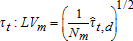 .
.
Data and Data Processing
We analyze 11 different futures markets that can be categorized into five commodity groups: grain (corn, soybeans, wheat); livestock (live cattle, lean hogs); energy (crude oil, natural gas, heating oil); precious metals (gold, silver); and industrial metals (copper). Futures price data present several advantages over cash price data. For example, they are available at a higher sampling frequency (daily rather than weekly), the futures contract is standardized (e.g. commodity grade), price discovery usually occurs in futures markets (9; 31), and futures are used as tools for hedging and for capitalizing on commodity price fluctuations.
 (4)
(4) and Fi,k,t is the commodity k's ith nearby futures price on day t. Thus, there are three price observations for each commodity on day t, resulting in contemporaneous correlation among the same-day observations. To correct for this correlation and use all three price observations on any given day, we apply the generalized least squares (GLS) method of 19.3 Briefly, the steps involve: (1) estimating the above regression model by ordinary least squares (OLS); (2) using the OLS residuals to compute sample means of associated squared residuals to obtain variance estimates of the first, second, and third nearby futures contracts, and to compute sample means of the products of related residuals to obtain estimates of covariances between first and second nearby, between first and third nearby, and between second and third nearby contracts; (3) computing the Cholesky decomposition of the variance-covariance matrix obtained in the previous step; (4) applying a GLS transformation to the data using the Cholesky decomposition; (5) estimating the regression model with the transformed variables via OLS; (6) eliminating insignificant regressors and repeating the same procedure with the new set of regressors. This way, we obtain contemporaneously-uncorrelated GLS residuals for each commodity to use in the spline-GARCH estimation.
To explain long-run economic determinants of volatility, we regress monthly low-frequency volatility obtained from the spline-GARCH estimation on both the fundamental macroeconomic variables that are common across commodities and the commodity-specific variables. Common macroeconomic variables include percentage changes in “Consumer Price Index for All Urban Consumers: All Items,” and “Industrial Production Index,” and the spread between the 10-year and 2-year “Treasury Constant Maturity Rate” obtained from ArchivaL Federal Reserve Economic Data (ALFRED). ALFRED is released by the Economic Research Division of the Federal Reserve Bank of St. Louis, and contains data on major economic variables available at the time of the release (without any revisions). All these variables are recorded monthly.4 We also include percentage changes in “Trade Weighted Exchange Index: Broad” obtained from the Board of Governors of the Federal Reserve System, which represents a weighted average of the foreign exchange value of the U.S. dollar against the currencies of a broad group of major U.S. trading partners.
For commodity-specific variables, we consider inventories for storable commodities. Even though gold and silver are storable, we could not obtain complete and reliable inventory data on these commodities. For corn, soybeans, and wheat we use the stocks-to-use ratio computed with the series of “Ending Stocks” and “Total Use” published in World Agricultural Supply and Demand Estimates (WASDE) reports released monthly by the World Agricultural Outlook Board of USDA. For live cattle, we compute monthly percentage changes in the number of cattle on feed released in Cattle on Feed reports by the USDA National Agricultural Statistics Service (NASS). For lean hogs, we interpolate quarterly percentage changes in the number of all hogs and pigs, computed using Hogs and Pigs reports released quarterly by the NASS, into monthly series with a step function. For inventories in energy markets, we use percentage changes in the monthly series of “U.S. Crude Oil Ending Stocks Excluding SPR,” “U.S. Natural Gas Underground Storage Volume,” and “U.S. Ending Stocks of Distillate Oil” series from the Energy Information Administration. Finally, for copper we compute percentage changes in the monthly series of “Stocks of Refined Copper in the United States” from the American Bureau of Metal Statistics.
Spline-GARCH Estimation
GLS-detrended residuals are first fitted to a conditional mean equation. Specifically, serial correlation is removed through a univariate ARMA filter, where the number of AR and MA terms is selected using likelihood ratio (LR) tests.5 After being filtered through the conditional mean equation, the residuals rt are fitted to the spline-GARCH model (1)–(3). The results presented in table 1 describe the GARCH model parameter estimates, robust standard errors (computed using the Bollerslev-Wooldridge method) and tests of significance, the preferred distribution of innovations (with degrees of freedom ν for the Student-t), the optimal number of spline knots k, and the half-life of shocks (in weeks) implied by the model.
| Corn | Soybeans | Wheat | Live Cattle | Lean Hogs | Crude Oil | Natural Gas | Heating Oil | Gold | Silver | Copper | |
|---|---|---|---|---|---|---|---|---|---|---|---|
| (a) Sample Period: 1990–2005 | |||||||||||
| α | 0.056 | 0.049 | 0.018 | 0.002 | 0.002 | 0.056 | 0.039 | 0.032 | 0.061 | 0.024 | 0.010 |
| [0.014] | [0.009] | [0.003] | [0.000] | [0.000] | [0.014] | [0.010] | [0.008] | [0.013] | [0.006] | [0.004] | |
| β | 0.788 | 0.903 | 0.197 | 0.878 | 0.967 | 0.787 | 0.898 | 0.905 | 0.877 | 0.959 | 0.962 |
| [0.045] | [0.017] | [0.045] | [0.280] | [0.036] | [0.045] | [0.023] | [0.022] | [0.018] | [0.090] | [0.016] | |
| k | 11 | 11 | 11 | 13 | 13 | 5 | 7 | 5 | 15 | 11 | 8 |
| ν | 2.883 | 3.234 | 4.957 | 2.746 | 3.943 | 2.883 | 2.878 | 3.711 | 2.723 | 2.782 | 3.267 |
| [0.139] | [0.187] | [0.149] | [0.121] | [0.076] | [0.140] | [0.150] | [0.228] | [0.146] | [0.147] | [0.187] | |
| λ G | 7.997 | 12.650 | 6.801 | 30.250 | 32.750 | 26.080 | 15.330 | 14.530 | 44.500 | 85.490 | 25.670 |
| λ | 0.816 | 2.822 | 0.090 | 1.092 | 4.448 | 0.816 | 2.122 | 2.133 | 2.158 | 8.201 | 4.982 |
| (b) Sample Period: 2006–2009 | |||||||||||
| α | 0.011 | 0.013 | 0.044 | 0.040 | 0.017 | 0.063 | 0.048 | 0.013 | 0.014 | 0.067 | 0.038 |
| [0.000] | [0.000] | [0.022] | [0.021] | [0.008] | [0.021] | [0.019] | [0.005] | [0.006] | [0.030] | [0.019] | |
| β | 0.952 | 0.373 | 0.847 | 0.873 | 0.908 | 0.885 | 0.416 | 0.963 | 0.552 | 0.675 | 0.831 |
| [0.000] | [0.189] | [0.096] | [0.091] | [0.011] | [0.040] | [0.018] | [0.048] | [0.094] | [0.143] | [0.078] | |
| k | 10 | 5 | 5 | 12 | 10 | 13 | 16 | 6 | 8 | 10 | 10 |
| ν | 8.658 | 6.747 | 6.049 | 2.613 | 6.768 | 8.878 | 4.650 | 8.106 | 4.971 | 3.568 | 4.914 |
| [3.786] | [1.475] | [1.125] | [0.243] | [2.386] | [2.308] | [0.423] | [1.915] | [0.695] | [0.394] | [0.544] | |
| λ G | 6.025 | 16.270 | 5.787 | 19.080 | 54.790 | 15.290 | 5.759 | 25.090 | 18.140 | 18.880 | 9.565 |
| λ | 3.628 | 0.146 | 1.201 | 1.531 | 1.784 | 2.562 | 0.181 | 5.704 | 0.243 | 0.465 | 0.988 |
- a
Note: λG is the half-life (persistence) of shocks, in weeks, for the baseline GARCH model, and λ is the half-life of shocks for the spline-GARCH model. Half-life is computed in business days as
 . Standard errors are given in brackets. Results for the standard GARCH model are available upon request.
The optimal number of knots ranges from 5 to 15 in the sample period 1990–2005, and ranges from 5 to 16 in the period 2006–2009. A smaller number of knots implies fewer but longer cycles in the low-frequency volatility component. For the period 1990–2005, volatility for energy commodities was clearly less cyclical than it was for agricultural commodities and gold, but this difference does not hold for the period 2006–2009. Spectral analysis on the spline cycles does not reveal economically meaningful findings.6 Likelihood ratio tests are used to obtain the most suitable error specification. A model using Normal errors is estimated as a restricted case against a model with Student-t errors, since the Gaussian Normal distribution is obtained from the Student-t as a limiting case (degrees of freedom  ). In all cases, the restriction of Normal errors is rejected by the LR test (see table 1). Similarly, for all commodities we cannot reject the GARCH(1,1) case as a restriction of higher-order GARCH specifications.
To evaluate the persistence of volatility shocks, their half-life is computed for all commodities in both sample periods and reported as the parameters λ and λG for the estimates from the spline-GARCH and standard GARCH models, respectively.7 Estimated using a standard GARCH model, volatility half-life in 1990–2005 ranges from a low of 6.8 weeks (wheat) to a high of 85.5 weeks (silver). However, when estimated using the spline-GARCH model, estimates of half-life drop substantially, ranging from a low of 0.1 week (wheat) to a high of 8.2 weeks (silver). From 2006–2009, half-life computed from a standard GARCH model ranges from 5.8 weeks (natural gas) to 54.8 weeks (lean hogs). Estimated from a spline-GARCH model, half-life drops to a range from 0.1 week (soybeans) to 5.7 weeks (heating oil). Indeed, volatility persistence computed from the spline-GARCH model is lower for all commodities in both sample periods. As noted by 14, allowing the unconditional variance to be time-varying through the τt term reveals shocks to be much less persistent than a benchmark GARCH model would suggest.8 This argument can be related to the work by 21, who showed that evidence of integrated conditional variance (i.e. permanent shocks, modeled as IGARCH) was spurious and disappeared once structural shifts in the unconditional variance were accounted for. Lastly, it appears that persistence increased for energy and decreased for metals during the commodity boom and bust cycle, but overall there is no clear evidence that persistence is greater for certain commodity groups.
To assess the improvement in goodness-of-fit provided by the spline-GARCH model, several standard metrics from the literature are considered (e.g. 16).9 First, as an in-sample tracking metric we compute the Root Mean Squared Error (RMSE) of the prediction error from using GARCH-implied conditional volatility (i.e. conditional standard deviation) to predict a proxy of realized volatility (i.e. the absolute value of GLS-detrended returns). We find that using the spline-GARCH model improves the fit for all commodities in both sample periods, reducing the prediction RMSE on average by 6.0% in period 1990–2005 and by 5.3% in period 2006–2009. Second, we compare R2 from regressions of realized volatility on conditional volatility provided by each model. We find that R2 increases for all commodities in both sample periods, with the exception of lean hogs. On average, R2 increases from 4.6% to 5.3% in the first sample period, and increases from 6.3% to 7.7% in the second sample period. The magnitudes of the goodness-of-fit metrics are comparable to 16 findings for equities. Third, we verify that both the model-implied unconditional volatility and conditional volatility match the sample unconditional volatility (i.e. standard deviation of returns or GLS residuals). Both GARCH models perform roughly as well in this regard. Fourth and last, using Kolmogorov and Ljung-Box tests, we confirm that the standardized innovations from the GARCH models are well-behaved (i.i.d. white noise) and both models perform well. Overall, the spline-GARCH model is a clear improvement over a standard GARCH model for goodness-of-fit and in-sample tracking.
Macroeconomic Determinants of Low-Frequency Volatility
 (5)
(5) (6)
(6) ,
,  ,
,  ,
,  take the value of one if the percentage change in the associated variable is nonnegative, and zero otherwise, while the indicator variables
  ,
,  ,
,  ,
,  take the value of one if the percentage change in the associated variable is negative, and zero otherwise. For corn, soybeans, and wheat the variable %ΔINVk,m refers to the stocks-to-use ratio in month m rather than the percentage change in inventories. Moreover, DSm is a summer dummy variable which takes the value of one if m is July, August, or September, and zero otherwise; DFm is a fall dummy variable which takes the value of one if m is October, November, or December, and zero otherwise; DWm is a winter dummy variable which takes the value of one if m is January, February, or March, and zero otherwise. We use this simple specification to account for seasonality because the commonly used alternatives, such as sinusoidal or polynomial functions, require higher-frequency observations. If inventory data are unavailable for a commodity, inventory terms are naturally excluded from the regression. Given K=11 commodities, M=189 months in the first sample period and M=47 months in the second, a total of 2,079 and 517 observations, respectively, are available in the SUR system. Results from the SUR estimation are presented in table 2. The table reports coefficient estimates and standard errors in brackets.10
| LV | Corn | Soybeans | Wheat | Live Cattle | Lean Hogs | Crude Oil | Natural Gas | Heating Oil | Gold | Silver | Copper |
|---|---|---|---|---|---|---|---|---|---|---|---|
| (a) Sample Period: 1990–2005 | |||||||||||
| Constant | 1.855*** | 1.615*** | 1.824*** | 1.009*** | 2.321*** | 2.146*** | 1.302*** | 1.883*** | 0.651*** | 1.397*** | 1.406*** |
| [0.101] | [0.093] | [0.090] | [0.064] | [0.138] | [0.166] | [0.093] | [0.146] | [0.069] | [0.104] | [0.074] | |
| %ΔCPI*I+ | 0.103 | 0.207 | 0.065 | −0.076 | −0.316 | 0.484 | 0.205 | 0.764*** | 0.150 | −0.184 | 0.181 |
| [0.144] | [0.153] | [0.116] | [0.111] | [0.225] | [0.296] | [0.158] | [0.261] | [0.126] | [0.190] | [0.136] | |
| %ΔCPI*I− | −0.156 | −0.115 | 0.099 | −0.131 | 0.677 | −0.656 | −0.443 | −1.929** | −0.530 | 0.030 | −0.279 |
| [0.430] | [0.457] | [0.345] | [0.332] | [0.674] | [0.884] | [0.471] | [0.779] | [0.374] | [0.568] | [0.401] | |
| %ΔIP*I+ | 0.126 | 0.114 | 0.062 | 0.063 | −0.112 | 0.013 | 0.138 | −0.036 | 0.034 | 0.089 | 0.169** |
| [0.088] | [0.094] | [0.071] | [0.068] | [0.138] | [0.182] | [0.097] | [0.160] | [0.077] | [0.117] | [0.082] | |
| %ΔIP*I− | −0.077 | 0.037 | −0.043 | 0.054 | −0.103 | −1.032*** | 0.057 | −0.807*** | −0.165* | 0.054 | 0.058 |
| [0.109] | [0.116] | [0.088] | [0.085] | [0.171] | [0.225] | [0.120] | [0.199] | [0.095] | [0.145] | [0.102] | |
| %ΔFX*I+ | −0.082** | −0.080** | −0.092*** | −0.054** | −0.102* | −0.103 | −0.087** | −0.073 | −0.017 | 0.029 | −0.050 |
| [0.036] | [0.038] | [0.029] | [0.028] | [0.056] | [0.074] | [0.039] | [0.065] | [0.031] | [0.047] | [0.033] | |
| %ΔFX*I− | 0.032 | 0.044 | −0.024 | −0.054 | −0.089 | −0.182* | 0.033 | −0.091 | −0.059 | −0.103 | 0.010 |
| [0.047] | [0.051] | [0.038] | [0.037] | [0.074] | [0.098] | [0.052] | [0.086] | [0.041] | [0.063] | [0.044] | |
| T-Spread | −0.076*** | 0.006 | 0.036 | 0.153*** | −0.042 | −0.254*** | 0.007 | −0.124** | 0.016 | 0.025 | −0.068** |
| [0.030] | [0.032] | [0.025] | [0.023] | [0.046] | [0.061] | [0.032] | [0.054] | [0.026] | [0.039] | [0.028] | |
| Summer | 0.089 | 0.096 | −0.133** | −0.128** | −0.011 | −0.074 | 0.240*** | 0.107 | 0.043 | −0.121 | −0.004 |
| [0.069] | [0.074] | [0.056] | [0.055] | [0.121] | [0.146] | [0.078] | [0.126] | [0.061] | [0.092] | [0.065] | |
| Fall | −0.326*** | −0.364*** | −0.323*** | −0.170** | −0.133 | 0.038 | −0.084 | 0.131 | 0.063 | −0.077 | 0.022 |
| [0.070] | [0.075] | [0.057] | [0.072] | [0.115] | [0.146] | [0.078] | [0.129] | [0.062] | [0.093] | [0.066] | |
| Winter | −0.439*** | −0.473*** | −0.128** | −0.050 | −0.059 | 0.337** | −0.339*** | 0.246* | 0.053 | 0.062 | 0.000 |
| [0.071] | [0.076] | [0.057] | [0.055] | [0.114] | [0.148] | [0.100] | [0.145] | [0.062] | [0.095] | [0.067] | |
| %ΔINV*I+ | −1.730*** | −1.347*** | −0.528** | −0.002 | −0.071*** | −0.054*** | 0.011 | 0.004 | −0.000 | ||
| [0.404] | [0.312] | [0.213] | [0.008] | [0.024] | [0.014] | [0.009] | [0.008] | [0.000] | |||
| %ΔINV*I− | 0.005 | 0.060* | 0.028* | 0.009 | 0.002 | 0.001 | |||||
| [0.009] | [0.034] | [0.016] | [0.011] | [0.008] | [0.002] | ||||||
| (b) Sample Period: 2006–2009 | |||||||||||
| Constant | 2.082*** | 1.474*** | 2.771*** | 1.014*** | 1.093*** | 0.823*** | 3.535*** | 1.279*** | 1.246*** | 2.195*** | 1.608*** |
| [0.171] | [0.359] | [0.286] | [0.125] | [0.329] | [0.230] | [0.641] | [0.147] | [0.194] | [0.373] | [0.273] | |
| %ΔCPI*I+ | 0.256 | −0.197 | 0.007 | 0.127 | −0.120 | 0.648** | −1.687** | 0.419** | 0.114 | −0.153 | 0.280 |
| [0.186] | [0.235] | [0.312] | [0.151] | [0.349] | [0.260] | [0.704] | [0.172] | [0.239] | [0.459] | [0.313] | |
| %ΔCPI*I− | −0.811*** | −0.339* | −0.293 | −0.304** | 0.321 | −1.977*** | 0.302 | −0.872*** | −0.663*** | −0.782* | −1.044*** |
| [0.163] | [0.206] | [0.275] | [0.132] | [0.313] | [0.232] | [0.625] | [0.161] | [0.211] | [0.405] | [0.276] | |
| %ΔIP*I+ | 0.202 | −0.050 | −0.176 | 0.285** | 0.270 | 0.494** | 0.509 | 0.200 | 0.044 | 0.548 | 0.778*** |
| [0.152] | [0.205] | [0.266] | [0.122] | [0.299] | [0.213] | [0.575] | [0.140] | [0.195] | [0.375] | [0.253] | |
| %ΔIP*I− | −0.161 | 0.084 | 0.006 | −0.153 | 0.065 | −1.100*** | −0.039 | −0.710*** | −0.165 | −0.189 | −0.738*** |
| [0.119] | [0.150] | [0.206] | [0.096] | [0.239] | [0.168] | [0.450] | [0.109] | [0.153] | [0.294] | [0.200] | |
| %ΔFX*I+ | 0.188*** | 0.314*** | 0.221** | 0.043 | −0.125 | 0.139* | −0.199 | 0.085* | 0.226*** | 0.511*** | 0.396*** |
| [0.056] | [0.072] | [0.096] | [0.045] | [0.108] | [0.079] | [0.214] | [0.051] | [0.072] | [0.139] | [0.094] | |
| %ΔFX*I− | 0.053 | −0.067 | −0.143 | 0.045 | 0.090 | 0.013 | 0.145 | 0.054 | 0.033 | −0.097 | −0.124 |
| [0.070] | [0.090] | [0.118] | [0.056] | [0.137] | [0.098] | [0.265] | [0.064] | [0.090] | [0.173] | [0.118] | |
| T-Spread | 0.120** | 0.346*** | 0.417*** | −0.012 | 0.383*** | 0.354*** | 0.224 | 0.252*** | −0.005 | 0.038 | −0.046 |
| [0.049] | [0.113] | [0.087] | [0.040] | [0.101] | [0.069] | [0.189] | [0.044] | [0.063] | [0.121] | [0.083] | |
| Summer | 0.239* | 0.286* | 0.024 | −0.102 | 0.345 | 0.200 | 1.255*** | 0.007 | −0.093 | −0.309 | −0.281 |
| [0.123] | [0.160] | [0.209] | [0.100] | [0.268] | [0.181] | [0.476] | [0.112] | [0.160] | [0.307] | [0.209] | |
| Fall | −0.143 | −0.350** | −0.081 | 0.041 | 0.453 | 0.128 | 0.711 | 0.110 | −0.262 | −0.745** | −0.142 |
| [0.136] | [0.175] | [0.231] | [0.152] | [0.286] | [0.200] | [0.527] | [0.133] | [0.176] | [0.339] | [0.237] | |
| Winter | −0.316*** | 0.029 | 0.084 | −0.196* | 0.715*** | 0.571*** | 1.921** | 0.377*** | −0.058 | −0.558* | −0.088 |
| [0.122] | [0.157] | [0.206] | [0.102] | [0.230] | [0.172] | [0.852] | [0.129] | [0.157] | [0.303] | [0.216] | |
| %ΔINV*I+ | −2.041*** | −1.156 | −4.314*** | −0.059** | 0.117* | 0.082** | 0.008 | 0.045*** | −0.003 | ||
| [0.782] | [1.606] | [0.865] | [0.023] | [0.071] | [0.034] | [0.079] | [0.017] | [0.007] | |||
| %ΔINV*I− | 0.016 | −0.328* | −0.021 | 0.269*** | −0.011 | −0.013 | |||||
| [0.018] | [0.167] | [0.033] | [0.104] | [0.015] | [0.010] | ||||||
- a Note: The model is estimated with the Seemingly Unrelated Regressions method. Standard errors are given in brackets, with *, **, and *** denoting significance at the 10%, 5%, and 1% levels, respectively.
-
(H1) Commodity price volatility is increasing in the absolute value of changes in the consumer price index (11).
-
(H2) Volatility is increasing in the absolute value of changes in the industrial production index (29).
-
(H3) Volatility is decreasing in changes in the trade-weighted foreign exchange index (25).
-
(H4) Volatility is decreasing in the U.S. Treasury interest rate spread (10-year to 2-year) (11).
-
(H5) Volatility is seasonal, with seasonal cycles that are commodity-specific and match both planting and harvest seasons (20).
-
(H6) Volatility is decreasing in inventories, implying that Working's theory of storage holds.
-
(H7) Volatility has a response that is asymmetric to negative and positive macroeconomic news (12).
-
(H8) All of these relationships are statistically equivalent within commodity groups, but statistically different across commodity groups.
-
(H9) Macroeconomic indicators have a greater effect on volatility during periods of higher volatility.
Low-Frequency Volatility from 1990–2005
Table 2(a) presents our results for the macroeconomic determinants of volatility in the first sample period of 1990–2005.11 Evaluating (H1), table 2(a) shows that coefficients on both positive and negative CPI changes are statistically significant only for heating oil in this period. A 1% increase in CPI (i.e. 1% inflation) leads to a 0.76 percentage point increase in the low-frequency volatility of heating oil, while a 1% decrease (i.e. 1% deflation) leads to a 1.93 percentage point increase in volatility. The magnitude of the change in volatility is greater for negative changes in CPI, supporting (H7). For most commodities though, coefficients are not statistically significant, and we find that volatility is increasing in the absolute value of changes in CPI (i.e. both inflation and deflation). Although a clear link between commodity dynamics and inflation has proven difficult to establish empirically, recently 15 have shown that the commodity convenience yield is remarkably linked to inflation; their research and others' suggest that overall, at least for storable commodities, the expected sign of inflation (i.e. percentage changes in CPI) on volatility is positive when inflation is positive, but negative when inflation is negative. That is, volatility is expected to be increasing in the absolute value of inflation, the latter being a proxy for inflation uncertainty. 14 indeed find that low-frequency volatility for equities worldwide is increasing in inflation volatility. Note, however, that our specification has the advantage of allowing the magnitude of the effect to be asymmetrical.
Regarding (H2), a 1% increase in the industrial production (IP) index increases the volatility of copper by 0.17 percentage point, while a 1% decrease in IP increases the volatility of crude oil, heating oil, and gold by 1.03, 0.81, and 0.16 percentage points, respectively. This suggests industrial metal markets are more volatile during economic booms, while energy and gold markets are more volatile during economic slowdowns. Across commodities, volatility tends to be increasing in the absolute value of changes in IP, though other coefficients are not statistically significant.
There is support for (H3), whereby volatility decreases when the trade-weighted exchange index (FX) increases in corn, soybeans, wheat, live cattle, lean hogs, and natural gas, as well as for crude oil, for which volatility increases when FX decreases. The largest effect is for hogs, where a 1% increase in FX decreases volatility by 0.10 percentage point. Results for other commodities, though less significant, generally support (H3).
In (H4) we consider the spread between the 10-year and the 2-year constant maturity rates, which can be seen as a proxy for the yield curve. The expected sign (negative), is confirmed for corn, crude oil, heating oil, and copper. Thus, volatility increases as long-term interest rates approach short-term interest rates. The largest effect, -0.25, is found for crude oil. The sign is, however, positive and large for live cattle. To see why the expected sign is negative, consider the term spread (or slope), and more generally the entire yield curve, which closely relates to the business cycle (e.g. 3). While premia are counter-cyclical for long-maturity treasury bonds, they are pro-cyclical for short bonds. Indeed, during recessions, investor risk-aversion drives up long bond yields, while short yields are reduced by the Federal Reserve. The term spread has been shown to have predictive power for real interest rates, GDP growth, business cycle indicators, and recessions. For instance, every recession after the mid-1960s has been preceded by a negative term spread (inverted yield curve), and only once has a negative slope not been followed by a recession. The literature therefore leads us to expect a negative sign on the term spread. This is because a negative spread likely implies a near-future recession and volatile commodity markets. A strongly positive spread, meanwhile, implies a near-future recovery from a current recession.
In (H5) we consider seasonality, and find that for corn, soybeans, and wheat, volatility is lower in the fall and winter compared to the spring baseline quarter. For live cattle, volatility is lower in the summer and fall. For crude oil and heating oil, volatility is higher in the winter, but for natural gas, it is higher in the summer and lower in winter. No significant seasonal effects are found for lean hogs or for any metals.
The theory of storage, (H6), whereby volatility is dampened by high inventory levels, is supported for corn, wheat, lean hogs, and crude oil. The effect is largest for corn. However, we also find that, for lean hogs and crude oil, volatility decreases as inventory levels decline.
Table 3 summarizes our findings for (H1)–(H6). The sign √ indicates that the empirical results presented in table 2(a) provide evidence to support these hypotheses at the 10% level, while the sign × indicates insufficient evidence. For variables allowing asymmetrical effects, the signs + and − are used to indicate empirical support. The inventory effect, (H6), is not tested for gold and silver because of the lack of inventory data. The table shows that, in the first sample period, the FX, seasonality, and theory of storage hypotheses are supported for many commodities, while the CPI, IP, and T-spread hypotheses are supported for a few commodities.
| H1 (CPI) | H2 (IP) | H3 (FX) | H4 (T-Spread) | H5 (Seasonality) | H6 (INV) | |||||||
|---|---|---|---|---|---|---|---|---|---|---|---|---|
| 1990–2005 | 2006–2009 | 1990–2005 | 2006–2009 | 1990–2005 | 2006–2009 | 1990–2005 | 2006–2009 | 1990–2005 | 2006–2009 | 1990–2005 | 2006–2009 | |
| Corn | × | − | × | × | + | × | √ | × | √ | √ | √ | √ |
| Soybeans | × | − | × | × | + | × | × | × | √ | √ | √ | × |
| Wheat | × | × | × | × | + | × | × | × | √ | × | √ | √ |
| Live Cattle | × | − | × | + | + | × | × | × | √ | √ | × | + |
| Lean Hogs | × | × | × | × | + | × | × | × | × | √ | + | − |
| Crude Oil | × | +,− | − | +,− | × | × | √ | × | √ | √ | + | × |
| Natural Gas | × | × | × | × | + | × | × | × | √ | √ | × | × |
| Heating Oil | +,− | +,− | − | − | × | × | √ | × | √ | √ | × | × |
| Gold | × | − | − | × | × | × | × | × | × | × | ||
| Silver | × | − | × | × | × | × | × | × | × | √ | ||
| Copper | × | − | + | +,− | × | × | √ | × | × | × | × | × |
- a Note: The sign √ indicates that empirical results provide evidence to support the associated hypothesis at the 10% level, and the sign × indicates that results provide no evidence to support the hypothesis. For variables with positive and negative changes, the signs + and − are used to indicate empirical support.
Results for (H7), which concerns the potentially asymmetrical effect of macroeconomic indicators on volatility, are summarized in table 4. A √ sign denotes rejection of the null hypothesis (equality of the estimated parameters on positive and negative changes), while the × sign denotes a failure to reject the null. Asymmetrical effects of inventory changes are not tested for grains and precious metals, and therefore represented by empty cells.12 There is significant evidence of asymmetrical effects for corn (FX), soybeans (FX), lean hogs (INV), crude oil (IP and INV), and heating oil (CPI and IP). Moreover, evidence supporting (H7) is much stronger in the second sample period (2006–2009), as described below.
| %ΔCPI | %ΔIP | %ΔFX | %ΔINV | |||||
|---|---|---|---|---|---|---|---|---|
| 1990–2005 | 2006–2009 | 1990–2005 | 2006–2009 | 1990–2005 | 2006–2009 | 1990–2005 | 2006–2009 | |
| Corn | × | √ | × | × | √ | × | ||
| Soybeans | × | × | × | × | √ | √ | ||
| Wheat | × | × | × | × | × | √ | ||
| Live Cattle | × | √ | × | √ | × | × | × | √ |
| Lean Hogs | × | × | × | × | × | × | √ | √ |
| Crude Oil | × | √ | √ | √ | × | × | √ | √ |
| Natural Gas | × | √ | × | × | × | × | × | √ |
| Heating Oil | √ | √ | √ | √ | × | × | × | √ |
| Gold | × | √ | × | × | × | × | ||
| Silver | × | × | × | × | × | √ | ||
| Copper | × | √ | × | √ | × | √ | × | × |
- a Note: The sign √ indicates a rejection of the null hypothesis of equality of the estimated parameters on positive and negative changes in the macroeconomic variables, and the sign × indicates a failure to reject the null hypothesis at the 10% level. Rejecting the null hypothesis provides evidence of asymmetric effects and support for (H7).
Low-Frequency Volatility from 2006–2009
Results for the second sample period, 2006–2009, are presented in table 2(b). There is now greater support for (H1), particularly for negative changes in CPI. Coefficients are significant for all commodities except for wheat and lean hogs. Volatility increases with deflation for corn, soybeans, live cattle, crude oil, heating oil, gold, silver, and copper, and increases with inflation for crude oil and heating oil. Curiously, volatility decreases with inflation for natural gas. The largest coefficient is found for crude oil, where a 1% decrease in CPI implies a 1.98 percentage point increase in volatility. Most coefficients are near but below −1.
The effect of IP changes, (H2), is also better supported in 2006–2009, with significant coefficients for live cattle, crude oil, heating oil, and copper. Volatility is increasing in positive IP changes for all but two commodities, and significant for live cattle, crude oil, and copper. It is also increasing in negative IP changes for all but three commodities, and significant for crude oil, heating oil, and copper. The largest effects are for copper, where a 1% increase in IP implies a 0.78 percentage point volatility increase, and for crude oil, where a 1% decrease in IP implies a 1.10 percentage point volatility increase.
For (H3), there is an unexpected reversal of the sign for the positive FX variable, with a positive and significant sign for corn, soybeans, wheat, crude oil, heating oil, gold, silver, and copper, while coefficients for a negative FX change are not significant. However, during 2006–2009 the U.S. dollar depreciated steadily, and the index itself was decreasing for 38 out of 47 months. The scarcity of periods during which the index was increasing may explain why our results are precisely the opposite of (H3).
Another surprising finding is that, for (H4), the T-Spread coefficient is significant and positive for most commodities. Thus, (H3) and (H4), which were validated in 1990–2005, show precisely the wrong sign in 2006–2009. The results imply that volatility is increasing as the spread between long- and short-term interest rates widen. A possible explanation is that short-term interest rates were maintained at an unusually low level by the Federal Reserve during the commodity boom that occurred prior to the financial crisis, whereas such monetary policy is normally reserved for recessions. The coefficient is significant for corn, soybeans, wheat, lean hogs, crude oil, and heating oil, and economically large and nearly significant for natural gas. Pointedly, it is very small and not significant for precious and industrial metals.
There is support for (H5), seasonality, for many commodities, particularly during the winter quarter for energy commodities. Surprisingly, no seasonal variables are significant for wheat.
The inventory effect, (H6), is supported for corn, wheat, and live cattle (volatility decreases as inventories, or stocks-to-use, increase), and for natural gas (volatility increases as inventories decrease). Coefficients are largest for corn (−2.04) and wheat (−4.31). The wrong sign is obtained for lean hogs, crude oil, and heating oil, but the coefficients for those commodities are very small and economically insignificant.
The results are summarized, alongside those for 1990–2005, in table 3. There is much greater support for the CPI hypothesis, while the IP, seasonality, and theory of storage hypotheses continue to be supported for many but not all commodities. Significant and opposite signs are obtained for most commodities for the FX and T-Spread hypotheses, suggesting that the unusual monetary situation of the United States from 2006–2009 (historically low short-run interest rates and a steadily depreciating U.S. dollar) complicates econometric inference.
The null of symmetrical effects is rejected much more frequently for 2006–2009, as table 4 shows, particularly concerning CPI. Energy commodities are the most likely to display asymmetrical effects.
Macro Effects within and across Commodity Groups
In (H8) we are concerned with whether the effects of macroeconomic variables vary within and across commodity groups. To evaluate (H8), we perform hypothesis tests on the estimated coefficients. Overall, we find that a greater number of macro effects are similar both within and across commodity groups during 1990–2005 than during 2006–2009. That is, we reject the null of equality of coefficients (within a group, or across groups) more frequently in the 2006–2009 period. More specifically, we restrict the coefficient estimate of a macroeconomic variable within a commodity group to be the same. For example, we restrict the  coefficient to be the same for corn, soybeans, and wheat (i.e. grain sub-group). Summary results are reported in table 5 for both sample periods. As before, the sign √ indicates a rejection of the null hypothesis of equality of estimated parameters within and across commodity groups, and the sign × indicates the failure to reject the null hypothesis at the 10% level. Inventory effects for precious metals are left empty due to a lack of inventory data on gold and silver.13 As the table shows, most of the within-group restrictions of macroeconomic variables hold for grain, livestock, and precious metals during the 1990–2005 period. Next, imposing within-group restrictions for all commodity groups at the same time, we test whether the parameter estimates across commodity groups are the same, for example, whether a positive CPI change affects commodities in all groups similarly. These results are presented in the column labeled “All” in table 5. Note that the tests on inventory coefficients exclude the grain commodity group, as the stocks-to-use ratio is used instead of inventory percentage changes. Furthermore, for all across-commodity group tests, copper is included to represent the industrial metals group.
| Grain | Livestock | Energy | Precious Metals | All | ||||||
|---|---|---|---|---|---|---|---|---|---|---|
| 1990–2005 | 2006–2009 | 1990–2005 | 2006–2009 | 1990–2005 | 2006–2009 | 1990–2005 | 2006–2009 | 1990–2005 | 2006–2009 | |
| %ΔCPI*I+ | × | × | × | × | √ | √ | √ | × | × | × |
| %ΔCPI*I− | × | √ | × | √ | √ | √ | × | × | × | √ |
| %ΔIP*I+ | × | × | × | × | × | × | × | √ | × | × |
| %ΔIP*I− | × | × | × | × | √ | √ | × | × | √ | √ |
| %ΔFX*I+ | × | × | × | × | × | × | × | √ | √ | √ |
| %ΔFX*I− | × | √ | × | × | × | × | × | × | × | × |
| T-Spread | √ | √ | √ | √ | √ | × | × | × | √ | √ |
| %ΔINV*I+ | √ | √ | √ | √ | √ | × | × | √ | ||
| %ΔINV*I− | × | √ | × | √ | × | × | ||||
- a Note: The sign √ indicates a rejection of the null hypothesis of equality of the estimated parameters within and across commodity groups, and the sign ×indicates a failure to reject the null hypothesis at the 10% level. The column labeled “All” shows test results for across-group restrictions, and includes the industrial metal group as well. The grain group is excluded in the test of %ΔINV parameters across groups. Failure to reject the null hypothesis within commodity groups and rejecting the null hypothesis across commodity groups provides support for (H8).
Lastly, we consider (H9), whether macroeconomic determinants have a greater effect in a high-volatility regime (period 2) than in a low-volatility regime (period 1). Based on the results presented in tables 2–5, we conclude that the evidence supports (H9): macro effects are more significant during exceptionally volatile periods. Moreover, effects tend to be more commodity-specific during volatile periods, and more common across commodities during less volatile periods.
Realized Volatility
Equation (5) was also estimated using realized volatility RVk,m as the dependent variable for both sample periods.14 There is less empirical support for (H1)-(H6) using realized volatility, especially for FX and inventories for the first sample period and CPI in the second sample period. There is also weaker evidence of asymmetrical effects (H7), especially for inventories. Lastly, within-group restrictions hold more for grain, energy, and precious metals, but less for livestock, while the equality of macro effects across commodity groups is rejected more often.
Using low-frequency volatility (LVk,m) rather than realized volatility as regressand therefore reveals more clearly the influence of macroeconomic indicators. This is because monthly RVk,m reflects substantial idiosyncratic daily price variation that obscures variation which is due to fundamentals. Although realized volatility, computed from sums of intra-daily return data, can provide accurate estimates of the true, unobservable volatility, it is sensitive to the choice of sampling window (Barndorff-Nielsen and Shephard 2004; 2).15
Conclusions
Economic theory suggests that commodity price volatility is affected by macroeconomic forces as well as by high-frequency market news. However, because macroeconomic indicators are sampled only monthly or quarterly, while prices are sampled daily or intra-daily, most empirical studies model volatility as being determined only by high-frequency news. In contrast, the present work estimates a model of high- and low-frequency volatility components for eleven commodities over the period 1990–2009, and relates the low-frequency component to data on macroeconomic indicators. To this end, we build on the spline-GARCH framework of 14, who studied international equities. A GLS-detrending procedure is used to obtain contemporaneously-uncorrelated price residuals to avoid the “splicing bias” associated with futures data, and a SUR framework is used to test several hypotheses on the macroeconomic determinants of commodity volatility.
We find that computing monthly volatility from the low-frequency component of volatility, rather than using realized volatility, reveals more clearly the effect of macroeconomic indicators, which supports 14 results on equities. Moreover, the effect of macroeconomic variables has been greater during the commodity bull-and-bear cycle than prior to it. Furthermore, a greater number of macro effects are common across commodities from 1990–2005, while they tend to be commodity-specific from 2006–2009. We also find that using a spline-GARCH model improves goodness-of-fit for daily volatility estimation and tracking, and reveals that volatility persistence is much lower than a standard GARCH model would imply.
For most commodities, low-frequency volatility is affected by changes in inflation, industrial production, inventories, and the long-term and short-term interest rate spread, especially during periods of high volatility. The effect is asymmetrical in some cases. Volatility for most commodities increases with both positive and negative changes in inflation and the industrial production index, and also with the interest rate spread. We also find that the effect of macroeconomic indicators generally does not vary within commodity groups, with the exception of inventories and the interest rate spread. Further research could investigate the model's implications for commodity option-pricing and price risk management, as well as for accuracy in long-term volatility forecasting (e.g. 13).
The authors acknowledge constructive comments from Wally Thurman, two anonymous reviewers, and the editor. The authors also gratefully acknowledge financial support from NIFA (formerly CSREES) Hatch project RI-9262, Institut de Finance Mathématique de Montréal (IFM2), and the Centre Inter-universitaire de Recherche sur le Risque, les Politiques Économiques et l'Emploi (CIRPEE).
 , and the unit is business days.