Modeling Grassland Conversion: Challenges of Using Satellite Imagery Data
Benjamin Rashford ([email protected]) is Associate Professor, Department of Agricultural and Applied Economics, University of Wyoming. Shannon Albeke ([email protected]) is Research Scientist, Wyoming Geographic Information Science Center, University of Wyoming. David Lewis ([email protected]) is Associate Professor, Department of Economics, University of Puget Sound.
This article was presented in an invited paper session at the 2012 AAEA annual meeting in Seattle, WA. The articles in these sessions are not subjected to the journal's standard refereeing process.
Conversion of native land cover to intensive agricultural production is one of the primary global threats to ecosystem and biodiversity conservation. The threat of conversion is perhaps most severe in temperate grasslands, which have the highest ratio of converted to protected area of any major biome (Hoekstra et al. 2005). Despite many proactive environmental policies (e.g. Grassland Reserve Program), U.S. temperate grasslands continue to face high conversion risk (Rashford, Walker and Bastian 2010). Conserving grasslands requires an understanding of the behavioral drivers of agricultural land-use conversion, and a wealth of economic literature has established the theoretical and empirical foundations for land-use decision-making (e.g. Lubowski 2002). Empirical models that include grassland, however, have been limited by data availability.
Most empirical models have relied on either aggregate data (e.g. Rashford, Bastian and Cole 2011) or National Resources Inventory (NRI) data (e.g. Rashford, Walker and Bastian 2010). These data sets offer limited ability to model grassland because: 1) they do not include explicit observations of grassland (i.e. they observe managed land uses correlated with grassland, such as pasture); and 2) they lack the spatial detail necessary to model grassland conversion at ecological and policy-relevant scales.
Land-use data derived from satellite imagery (or remote sensing) now offers an alternative to aggregate and NRI data. The Cropland Data Layer (CDL) produced by U.S. Department of Agriculture National Agricultural Statistics Service (USDA NASS) is perhaps the best dataset for examining agricultural land-use in the United States. The CDL uses satellite imagery combined with ground surveys to identify land-use/land-cover with continuous spatial coverage at a resolution of 900 m2 plots (i.e. approximately 4 plots per acre). The data classifies land cover into 135 categories, including explicit agricultural uses (e.g. corn), natural land covers (e.g. shrubland), and developed land uses. Thus, CDL data allows modelers to more explicitly identify grassland land-use. Additionally, since the CDL is a longitudinal survey with contiguous spatial coverage, modelers can: 1) identify explicit land-use transitions; 2) include fine-scale predictors of land-use (e.g. plot-level soil and climate characteristics; and 3) predict the spatial pattern of land use.
The high resolution of satellite imagery data, however, raises several computational and empirical challenges. The resolution implies a very large sample for all but the smallest geographic extent. For example, our model of land use in the Northern Great Plains (NGP) described below includes 154 counties with approximately 139 million plot-level observations. Most personal computers are not capable of storing, let alone manipulating, such a large database. Similarly, standard statistical software is not designed to estimate models with so many observations.
Empirical models using satellite imagery data are also likely to suffer from several statistical issues. Spatial dependence may be the most problematic of these to address (see Lubowski 2002 for a discussion of issues in plot-level panel data models). There are many reasons why plots may be spatially dependent, such as sharing correlated unobservables (e.g. common zoning). High-resolution satellite imagery data on agricultural land-use, however, is almost sure to generate spatial dependence. The scale of plots is smaller than the scale over which land-use decisions are made (i.e. ownership parcels are larger than plots). Land-use decisions on one plot are therefore influenced by the decisions on nearby plots. As a result, plot-level observations of land use will be spatially autocorrelated (i.e. spatially lagged). In the case of discrete choice models, which are typically used to empirically model land use, spatial autocorrelation can lead to both inconsistent and inefficient parameter estimates (Beron and Vijverberg 2004).
We consider these challenges in a model of grassland and cropland in the NGP. Specifically, we use alternative sampling methods within a bootstrapped estimation procedure to demonstrate the computational and statistical tradeoffs inherent to using high-resolution satellite imagery data in empirical land-use models.
Modeling Grassland Conversion Using Satellite Imagery Data
We use 2009 CDL data to identify land use in the NGP. Since our focus is on cropland and grassland, we aggregate the CDL classes into these two cover types. All other cover types are omitted (e.g. open water and developed). We also omit all public and tribal land plots since a different process likely drives their land-use. The resulting data set contains 139,569,983 observations (67% of the total area), with approximately 102.5 million grassland plots and 37.1 million cropland plots.
 (1)
(1) (2)
(2)We use data from the U.S. Department of Agriculture Economic Research Service to construct county-level cropland net returns by using an area-weighted average of returns less operating costs. Land capability class (LCC) is a composite index of the soil's productivity in agriculture, with LCC 1 being the highest productivity and LCC 8 the lowest (Soil Survey Staff 2011). We interact LCC with county-level net returns to scale returns up or down according of the productivity of each plot (see Lewis and Plantinga 2007). We then use census data on total direct government payments less conservation payments to form the governmental payments variable. All returns data are converted to expectations using a one-year lagged, five-year average. Finally, we construct a dryness index (growing season degree days per year >5°C/growing season precipitation) using data from the Rocky Mountain Research Station to capture spatial variation in historical average weather conditions (Crookston and Rehfeldt 2010). Since the final dataset is too large (approximately 96.8 GB) to manipulate on a standard personal computer with standard software (e.g. Microsoft Access has a file limit of 2GB), we store the data on a server using Microsoft TMSQL server software, which provides the capacity to store and manage data tables as large as 16 terabytes. We estimate models using 64 bit R, version 2.13.1 (R Development Core Team 2010).
Alternative Estimation Approaches and their Implications
We use a bootstrap regression approach to estimate the binary logit model (see Efron and Tibshirani 1993). The standard bootstrap approach is to: 1) draw a sample (Sj) of size n from the full data set; 2) run the binary logit model on Sj and retain the parameter estimates; 3) repeat steps 1 and 2 k times (i.e. draw j=1,…k samples); and 4) derive the bootstrapped parameter estimates and standard errors across k (e.g. average across the k samples). Several questions arise when applying this procedure to the CDL dataset, including how to draw samples, and how to choose n and k.
Sampling Strategies to Reduce Computational Constraints
First, standard bootstrap techniques suggest that samples should be drawn randomly, such that each observation has the same probability of being drawn, and that each sample be the same size as the original data. Following these procedures is untenable in our case. Logit models are sensitive to the proportion of outcome events observed in the sample, and can generate inconsistent estimates if too few of one event is observed (see e.g. King and Zeng 2001). Thus, for relatively small n, random sampling could generate samples with too few observations of cropland or grassland plots. The chance of drawing extremely unbalanced samples, or of any one sample affecting the bootstrapped estimates, vanishes as n and k grow arbitrarily large; a fact which provides little solace to those searching for computationally feasible approaches. Moreover, since the specification in (2) includes dummy variables, estimation will be infeasible unless each category of the dummy variables is observed in each sample. Lastly, drawing samples that are the same size as the original data set (i.e. 139 million) is clearly computationally infeasible.
One approach to address these sampling problems is to use a stratified random sampling procedure to draw samples that are consistent with the original data set and are computationally feasible. Specifically, one would stratify the data on the dependent variable (i.e. cropland and grassland) and dummy variables, then draw samples such that the proportion of each strata within each sample is equal to the proportions observed in the full data set. Since this sampling maintains the full sample proportions of the dependent variable, it does not constitute endogenous sampling and therefore does not bias parameter estimates (see Cameron and Trivedi 2005, p. 822).
Although the simple stratified sampling approach generates consistent parameter estimates, it is computationally intensive. In our case, drawing a stratified random sample from the full data set and estimating the model required slightly over one hour of processing time (regardless of n), which quickly becomes infeasible for large k (e.g. k=5,000 implies over 200 days of processing).2 An alternative approach is to reduce the number of observations by removing duplicates. Specifically, of the approximately 139.6 million observations in our data, only 2,287,344 observations are wholly unique (i.e. the specific combination of all variables is never replicated). Thus, aggregating the data by removing all “duplicates” can greatly reduce the number of observations.
The probability of observing any given plot in this “aggregated” sample, however, is not the same as drawing from the full dataset. Aggregating is therefore equivalent to endogenously sampling–since plots that are more “common” are essentially under-sampled–which induces endogeneity and therefore inconsistent parameter estimates (Cameron and Trivedi 2005, p. 824). The characteristics of the full sample, and hence consistent parameter estimates, can be estimated from the aggregated data by using weighted maximum likelihood, where the weights correct for the number of times each observation in the aggregated sample is observed in the full data set.
We therefore use the weighted estimation approach to generate consistent parameter estimates, which can be compared to standard sampling procedures. Specifically, we aggregate the data, and then perform the bootstrap estimation procedure described above with observations in each bootstrap sample (j=1,…,k), weighted by the number of observations in the full dataset with the characteristics of plot i.
Bootstrapped estimates from the full and aggregated datasets are not statistically different (α=0.05) when appropriate samples are compared. For example, consider the estimated marginal effect of government payments, which is the least stable variable in the model (figure 1). Even at large k, the estimated marginal effects do not statistically differ across sampling strategies. This suggests, as expected, that the aggregated sample with sufficient n and k will generate estimates that approximate those that would occur if samples were drawn from the full dataset. Moreover, the aggregated data has a distinct computational advantage–sampling from the aggregated data can produce 90 bootstrapped models per minute, compared to approximately one model per hour with the full dataset.
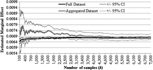
Bootstrapped marginal effect of government payments for alternative sampling procedures
This brings us to the question of how to choose n and k. Recall that standard bootstrap procedures involve drawing samples of equal size to the original, which negates any need to choose an appropriate n. Instead, the focus is on choosing the number of samples (k) to achieve a pre-determined level of precision (see e.g. Ross 2002, p. 113). In our sampling procedure, however, both n and k must be chosen. To understand the empirical and computational tradeoffs of this choice, we compare bootstrapped estimates for alternative values of n and k.
As n increase, bootstrapped estimates tend to converge asymptotically towards the same value (figure 2). For small n, however, some estimates converge to statistically different values than their larger sample counterpart. Though small in absolute magnitude, these differences can be policy-relevant. Consider the predicted impact of a $10 increase in government payments. Simply predicting from the means of the data indicates that policy predictions from a small sample can be orders of magnitude different from those in larger samples (table 1). A reasonably large sample with n=1,200, for example, would predict approximately 200,000 more acres of new cropland than would be predicted from samples with n>12,000.
| Sample size (n) | ||||||||
|---|---|---|---|---|---|---|---|---|
| Sample size (n′) | 300 | 600 | 1,200 | 3,000 | 6,000 | 9,000 | 12,000 | 15,000 |
| 600 | 28% | |||||||
| 1,200 | 34% | 20% | ||||||
| 3,000 | 38% | 25% | 15% | |||||
| 6,000 | 40% | 27% | 17% | 9% | ||||
| 9,000 | 40% | 27% | 17% | 8% | 3% | |||
| 12,000 | 41% | 28% | 18% | 10% | 4% | 1% | ||
| 15,000 | 41% | 29% | 19% | 10% | 5% | 2% | 1% | |
| 18,000 | 42% | 29% | 19% | 11% | 5% | 2% | 0% | 1% |
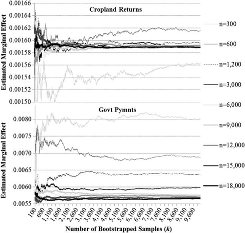
Bootstrapped marginal effects across alternative sample sizes (n) and number of bootstrapped samples (k)
Bootstrap accuracy is also affected by sample size, with estimates from larger samples converging more quickly (figure 3). Thus, small samples, even if they produced estimates consistent with the full dataset, require significantly more bootstrapped samples to achieve the same level of precision as larger samples (i.e. similar confidence intervals). In terms of computational time, drawing additional samples is more costly than drawing larger samples. Thus, our results suggest that modelers are better off choosing a larger n, and then choosing the k that achieves the level of precision necessary for the context. In our case, models with n≥9,000 (0.4% of the aggregated dataset) all converged to essentially the same parameter estimates around k=5,000, beyond which additional samples do not significantly improve precision. Our largest sample (n=18,000), however, produced the same parameter estimates and level of precision with k=1,418.
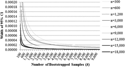
Width of 95% confidence interval for marginal effect of government payments across alternative sample sizes (n) and number of bootstrapped samples (k)
Sampling to Address Spatial Autocorrelation
Although recent advances have resulted in tests and corrections for spatial autocorrelation in limited dependent variable models (see Schnier and Felthoven 2011), options are limited for logit models, and even more limited in the context of large datasets. Approaches to correct for spatial dependence using a spatial weights matrix, which relates the errors at each location to the errors at every other location, are not computationally feasible in large plot-level datasets (Lubowski 2002). An alternative approach is to purge the data of spatial dependence by only sampling spatially distant observations (e.g. Munroe, Southworth, and Tucker 2002).
In most applications, the drawback of spatial sampling is that it implicitly reduces the number of observations. This is not an issue with large datasets or with a bootstrapped estimation procedure. Instead, the drawback is computational time. With our full dataset (n≈139 million), drawing a spatially-corrected stratified random sample and estimating a single model requires nearly 1.5 hours. We cannot spatially sample from the smaller aggregated dataset, which would be substantially faster, since the spatial relationship between plots is lost in the aggregation process. To explore the potential implications of spatial sampling, we sampled (k=1,900 for computational ease) from our full dataset using a spatial restriction of two miles, which ensures that plots are further apart than the average farm size in the region.
Comparisons between bootstrapped parameter estimates for spatially and non-spatially sampled models suggest that spatial sampling affects parameter estimates. Some parameters converge to estimates that are not statistically different (e.g. marginal effect of crop returns), while others (e.g. marginal effect of annual dryness) are statistically different (figure 4). The non-spatially sampled bootstrapped estimates, when significantly different, tend to systematically underpredict parameter estimates. Differences between the spatially and non-spatially sampled models suggest that spatial autocorrelation may be affecting the consistency of parameter estimates in the non-spatially sampled models. Addressing spatial dependence with spatial sampling is, however, practically intractable given the required computational time.
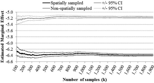
Bootstrapped estimates of the marginal effect of dryness for spatially and non-spatially stratified samples
Conclusions
While satellite imagery data has great promise for improving empirical models of grassland (and other natural land) conversion, more investments are needed to develop efficient methods for addressing the computational challenges of large plot-level datasets. Stratified sampling and bootstrapped estimators can be a computationally feasible approach, but the number of observations in each bootstrapped sample and the number of samples used cannot be arbitrarily chosen. Our results suggest that parameter estimates are significantly influenced by the size of bootstrapped samples, with small samples converging to statistically and practically different estimates than larger samples, even when a large number of samples are used. Since drawing large samples is less computationally costly than drawing multiple samples, we suggest modelers error towards the largest sample size that is computationally feasible.
Our results also suggest that aggregating the data by eliminating duplicate plots and using a weighted estimator can substantially reduce computational constraints. Aggregating the data, however, eliminates the ability to use spatial sampling to reduce spatial autocorrelation. This is particularly problematic given that our spatially sampled bootstrap estimates generate significantly different estimates than those from non-spatially sampled models. While addressing spatial autocorrelation appears necessary, the computational time required for spatial sampling (1.5 hours per sample) is nearly intractable in a bootstrap context.
A final issue with satellite imagery that we did not address in this contribution is remote sensing accuracy. Satellite imagery data are the result of a model (i.e. an empirical model translates the satellite images into plot-level data). As such, the dependent variable suffers from measurement error. Moreover, since the measurement error is not necessarily random (i.e. some land uses are more accurately identified than others), empirical models that ignore accuracy and the associated error propagation may draw an incorrect inference–particularly as it relates to the efficiency of parameter estimates and predictions. Future work should therefore explore the implications of remote sensing accuracy for parameter estimates in empirical land-use models.


