The mid-domain effect cannot explain the diversity gradient of Nearctic birds
Abstract
A recent explanation for diversity gradients proposes a ‘null model’ based on how species ranges are constrained by the geometry of bounded domains. We conduct a test of this hypothesis by comparing patterns predicted by two two-dimensional geometric models against observed diversity patterns for terrestrially feeding Nearctic birds. Consistent with previous tests in two-dimensional space, we find empirical support for the hypothesis to be very weak. We also point out a fundamental conceptual flaw in the hypothesis with respect to the key assumption that ranges can exist independently of the environment in which they are embedded that undermines its theoretical basis as well. We conclude that the mid-domain effect has little empirical support and no theoretical support for its existence, and recommend that it be eliminated as a potential explanation for diversity gradients.
Introduction
Understanding patterns in the geographical distribution of species diversity presents ecology and biogeography with perhaps their greatest challenge, and attempts to identify potential mechanisms that date back almost 200 years (von Humboldt, 1807). However, research over the past 20 years has greatly reduced the number of probable explanations to far fewer than the 30 + hypotheses that have been proposed (Rahbek & Graves, 2001). A recent addition to the list, the mid-domain effect (Willig & Lyons, 1998; Lees et al., 1999; Colwell & Lees, 2000) argues that diversity gradients can arise from geometric constraints on how ranges can be distributed in bounded ‘domains’ independently of any environmental gradients, and that this mid-domain effect represents a ‘null model’ for diversity patterns. Attempts are now being made to test to what extent geometry actually accounts for observed diversity patterns.
The initial models of the mid-domain effect as an explanation for large-scale diversity gradients were generated in one-dimensional space and focused on latitude (Willig & Lyons, 1998; Colwell & Lees, 2000; Koleff & Gaston, 2001; but see Colwell & Hurtt (1994) and Rahbek (1997) for earlier applications of the idea to other types of uni-dimensional diversity gradients). However, such models ignore the fact that terrestrial species are distributed in two dimensions and that geometric models must explain longitudinal as well as latitudinal gradients (Bokma & Mönkkönen, 2000). Consequently, attention is now focused on generating two-dimensional models and comparing them to observed diversity patterns. To date, three such tests have been conducted at continental and intercontinental extents (Bokma et al., 2001; Jetz & Rahbek, 2001; Diniz-Filho et al., 2002). In all cases, fits of data to the models were poor, with coefficients of determination ranging from < 5% for South American raptors (Diniz-Filho et al., 2002), 8.5% for New World mammals (Bokma et al., 2001) to < 26% for Afrotropical birds (Jetz & Rahbek, 2001). This contrasts sharply with similar analyses of regional-scale diversity patterns using climatic and/or topographical predictors that typically generate coefficients of determination greater than 70% (e.g. Richerson & Lum, 1980; Currie & Paquin, 1987; Turner et al., 1987; Adams & Woodward, 1989; Currie, 1991; Guégan et al., 1998; Roy et al., 1998; Rutherford et al., 1999; Boone & Krohn, 2000; O’Brien et al., 2000; Balmford et al., 2001). However, despite the relatively poor fit of real diversity gradients with geometric null models so far and consequently little empirical support for the hypothesis, the mid-domain effect has been included recently in a list of five ‘credible’ hypotheses for diversity gradients (Rahbek & Graves, 2001).
In this paper we test further the credibility of the mid-domain effect as an explanation of diversity gradients using both empirically and theoretically based arguments. The empirical test uses the terrestrial breeding birds of the Nearctic biogeographical region. Because the logic of the hypothesis requires that species ranges have to be found entirely within the domain, we restrict the analysis to those species whose breeding ranges are confined to continental Canada, the United States and northern Mexico, the latter representing an approximate southern geographical limit to the Nearctic (see Fig. 1). This definition of domain assumes hard boundaries at the northern, eastern and western limits (the oceans) and a soft boundary to the south (a tropical climate). Climate is considered acceptable for delimiting domains (Colwell & Lees, 2000), and the fact that biogeographers divide the New World into the Nearctic and Neotropical regions is prima facie evidence that species dispersal between North America and Central/South America has been constrained historically by one or more barriers.
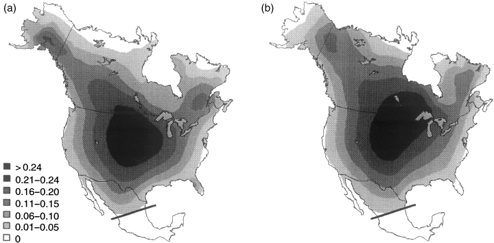
Diversity gradients (measured as the proportion of the regional species pool) predicted by two geometric models. a: The Willig & Lyons model extended into two-dimensional space (WL2D). b: The area-corrected two-dimensional model (AC-WL2D).
Our empirical test of the mid-domain effect is based on the analytical null model of Willig & Lyons (1998), extended first into bi-dimensional space and then corrected for area effects. We selected this approach because of the difficulties associated with creating biologically realistic bi-dimensional geographical ranges adequate for use in randomization procedures (Bokma & Mönkkönen, 2000; Colwell & Lees, 2000; Koleff & Gaston, 2001). This model also has critical underlying assumptions about species ranges, i.e. that there is a uniform distribution of geographical range midpoints and that the maximum possible range of a species is equal to the full area of the domain. Even so, this basic approach is useful because of its computational simplicity and ease of interpretation.
Our theoretical argument is based on the realization that the hypothesis assumes that range sizes are a fixed property of the organism rather than the actual situation that observed ranges are the product of an organism–environment interaction. We will argue that once this is realized, there is no theoretical basis for a mid-domain effect in either the real world or in hypothetical worlds without climatic gradients. We first present and discuss the empirical analysis, followed by the presentation of the theoretical argument.
Methods
Bird species richness
Bird richness estimates were generated by overlaying a grid system of 359 sample points equally spaced 220-km apart over the breeding distribution maps in Howell & Webb (1995) and National Geographic Society (1999). The use of sample points differs from most continental-extent analyses of diversity gradients, but because the mid-domain effect predicts point diversities rather than area diversities, point estimates were taken to allow comparison between predicted and observed values. This generated lower richness estimates than would a cell-based sample system, but it does not influence the geographical pattern of diversity. In total, 252 species of terrestrially feeding birds were included in the analysis. The observed diversity gradient was generated simply by recording whenever a sample point was within a species’ reported range. Because it has been argued that species with large ranges should be more influenced by geometric constraints than species with smaller ranges (Colwell & Lees, 2000; Jetz & Rahbek, 2001), we also classified birds into three classes, 177 species with small ranges (< 25% of the sample points), 65 species with intermediate ranges (between 25% and 50% of the sample points) and 10 species with large ranges (> 50% of the sample points), and compared the model fit for each class separately as well as for all birds considered together.
The geometric models
In the uni-dimensional (latitudinal) version of the null model (Willig & Lyons, 1998), the species richness at a point P, defined by a pure stochastic process, is a function of its distance to northern and southern endpoints of the continent, defined by the proportions p and q. The species richness in P is then given by 2pqS, where S is the total species richness in the continent (the species pool). Bokma et al. (2001) extended this model to a bi-dimensional space by including relative distances from P to western and eastern continental boundaries (r and t). In this version, called here the WL2D null model, the species richness expected at P is then given by 4pqrtS. Bokma et al. (2001) also constructed a null model based on speciation, migration and extinction that produced results very similar to the WL2D model.
The values of p, q, r and t in the null model were calculated for each of the points of the grid by considering their positions relative to boundaries across north, south, east and west directions, respectively. Each of these values was estimated from each point to the immediate continental boundary, such that continent shape has a direct effect on the expected richness, as in the evolutionary model of Bokma et al. (2001) and the spreading-dye model of Jetz & Rahbek (2001). Under this null model (and all similar geometric models), there is a diversity peak in the middle of the continent (Fig. 1a).
It is important to note that under this model, a peninsular region (e.g. Florida), that possesses a point that does not ‘contact’ the main body of the continent in all directions will have a large expected diversity, because the p, q, r and t proportions will be set in relation to the borders of the peninsula and not of the entire continent. Thus, in an irregularly shaped area such as North America high diversity points at the bases of peninsulas will be surrounded closely by lower diversity estimates, generating multiple secondary diversity peaks in the region (see Fig. 1a). To reduce this effect, we then also estimated p, q, r and t proportions based on the maximum north–south and east–west axes, creating an alternative null model. In this new null model, which we refer to as the ‘area-corrected’ version of Willig & Lyons’ (1998) model (the AC-WL2D model), the absolute distance of a point to the continental border is taken into account, correcting for available land area. This reduces the number of peninsular diversity peaks, although a secondary peak remains at the Alaskan–Canadian border (Fig. 1b).
We used the coefficients of determination (R2) between expected and observed species richness at each sample point to evaluate the agreement between the data and the two geometric models. As is widely appreciated, geographical data are not independent and are subject to strong autocorrelation effects, making significance tests too liberal (Bell, 2001; Jetz & Rahbek, 2001; Diniz-Filho et al., 2002). To examine the influence of spatial autocorrelation on statistical evaluation of the models, we initially used spatial correlograms, constructed using Moran's I coefficients estimated at distinct distance classes, for the species richness based on all species and species with small, intermediate and large geographical ranges. Moran's I coefficient is given as

where n is the number of points in the grid, yi and yj are the values of the variable (i.e. species richness) in the points i and j, ȳ is the average of y, wij is an element of the matrix W, which assumes a value of 1 if the pair i, j of points is within the geographical distance class interval. K is given by the count of these connections among points in W, for each class interval. We used 15 geographical distance classes. The value expected under the null hypothesis of no autocorrelation is given as −1/(n – 1). Detailed computations of the coefficient and of its standard error are given in Legendre & Legendre (1998).
Because significant autocorrelation patterns were found for all data subsets, regressions between observed and expected diversity were repeated using a generalized least squares (GLS) approach, incorporating in the error term of the regression equations the spatial covariance among observations (i.e. grid points), following Selmi & Boulinier (2001). Different models of spatial structure (spherical, Gaussian and exponential — see Legendre & Legendre, 1998) were tested, and the best fitting model was defined using the Akaike information criterion (Littell et al., 1996; Selmi & Boulinier, 2001). All these GLS procedures were implemented using the PROC MIXED routine in SAS (Littell et al., 1996).
Results
Endemic bird species richness reaches it highest levels in a broad latitudinal band extending across the entire region, being broadest in the Rocky Mountains (Fig. 2a). When birds are distinguished by the sizes of their ranges, the pattern for small-ranged species differs qualitatively from the pattern of intermediate- and large-ranged species. Whereas the former reach their greatest diversities in the eastern forests of the United States and in a narrow strip extending from Wyoming to coastal northern California (Fig. 2b), the latter form the basis for the overall pattern (Fig. 2c,d).
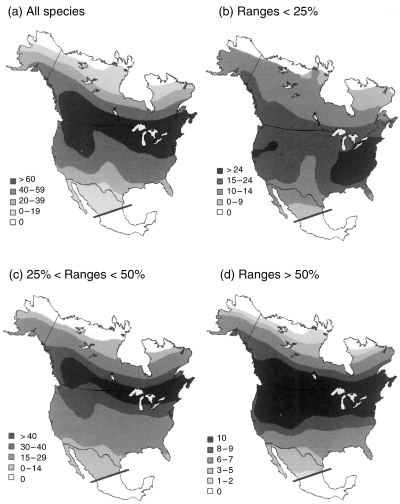
Diversity gradients for endemic terrestrial, breeding birds in the Nearctic region. (a) All species (s = 252). (b) Small-ranged species (s = 177). (c) Intermediate-ranged species (s = 65). (d) Large-ranged species (s = 10).
Moran's I coefficient indicated a significant spatial pattern in all diversity estimates (Fig. 3), with high positive autocorrelation in the shorter distance classes, but stabilizing when distances were greater than 10 points in the grid. Coefficients again increased at the largest distance classes, but they were always much smaller than coefficients in the first distance class, indicating a general trend to stabilization beyond 10–12 points in distance across the grid.
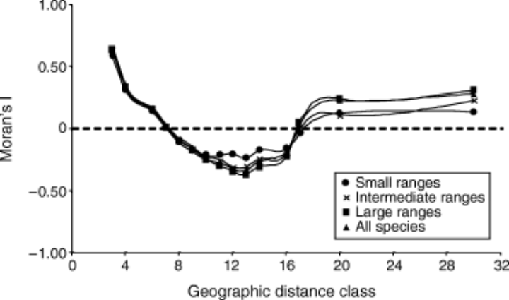
Spatial correlograms of species diversity in Nearctic birds, estimated for all species, small-ranged species, intermediate-ranged species and large-ranged species. Correlograms were defined by Moran's I coefficients in 15 geographical distance classes, indicating links among sampling points successively separated by 220 km in the grid.
The observed pattern of bird richness clearly varied from that predicted by both geometric models (cf. 1, 2), and coefficients of determinations are low irrespective of the sizes of ranges, based on standard regression analyses using ordinary least squares (Table 1). In both models, species with small ranges showed a much poorer fit than species with larger ranges, but in all cases the models explained less than 25% of the variance in observed bird species richness. The area-corrected model also always performed worse than the basic model (Table 1).
| Model | WL2D | AC-WL2D | ||||||
|---|---|---|---|---|---|---|---|---|
| R 2 | t(β = 0) | t(α = 0) | t(β = 1) | χ2 | R 2 | t(b = 0) | χ2 | |
| Bird richness | ||||||||
| All species | 0.206 | 3.6** | 0.2 | 13.5** | 756.8** | 0.166 | 1.6 | 764.8** |
| Small ranges | 0.052 | 1.3 | 1.8 | — | 573.8** | 0.022 | 0.9 | 585.0** |
| Intermediate ranges | 0.221 | 4.5** | 0.1 | 3.4** | 807.1** | 0.205 | 1.7 | 799.3** |
| Large ranges | 0.243 | 2.8** | 0.1 | 2.1* | 781.7** | 0.208 | 1.4 | 792.7** |
- * P < 0.05;
- ** P < 0.01.
As expected by the correlogram profiles, the best-fitting GLS model assumed an exponential decrease with the geographical distance in the error term matrix, according to the Akaike criterion. Also, in all cases, GLS models fit the data more effectively than non-spatial models and permitted initial statistical tests of regression slopes for β= 0 (i.e. there is no agreement between the data and the null model). For the WL2D model, slopes were significantly different from zero except when species richness includes only small-ranged species. When the null hypothesis of independence is rejected, then the regression line can be tested for α= 0 and β= 1, indicating no bias in model fit (see Jetz & Rahbek, 2001). The regression intercept was not different from zero in all cases, indicating no common bias across the range of diversity estimated by the null model (i.e. a good fit in overall magnitude). However, none of the slopes was equal to one (Table 1), indicating a poor fit in shape. For the null model corrected by peninsular effects (AC-WL2D), none of the slopes was statistically significant (Table 1).
Discussion
We find only very weak empirical support for the hypothesis that the diversity gradient of endemic birds in the Nearctic region is determined by ‘geometric constraints’ on species ranges. It also made little difference which null model we used. The original model (WL2D), despite possessing a statistically significant fit to data after correcting for spatial autocorrelation, had low explanatory power, accounting for only 21% of the variance across all species. The area-corrected model (AC-WL2D) performed even worse, having no significant fit to the observed richness patterns. The better fit of the former version can be explained mainly because there is a trend in the observed data of relatively high species richness toward southern Alaska, which also functions as a large peninsula. That the WL2D model fits the data at all is also influenced by an artefact arising from the delimitation of our domain. Endemic bird species richness decreases from central North America to Mexico, in apparent agreement with the predictions of the mid-domain effect. However, bird richness does not actually decrease into Mexico; this just appears to be the case because a large number of bird species in the west have ranges extending into the Neotropics, and therefore were excluded from the data. Maximum bird species richness in North America is actually found in the Sierra Nevada, the Transverse Ranges of southern California and in south-eastern Arizona (Cook, 1969), and if we were to extend the domain southward, the high-richness region becomes l-shaped, encompassing a band from New England westward to south-western Canada and then southward to northern Mexico. A concentration of bird species near the western edge of North America is unexpected under any geometric model irrespective of how the Nearctic domain is defined, and therefore extending the domain into Central America to incorporate these western birds would generate an even poorer fit than we already found.
Because the WL2D model does show a statistically significant association with bird species richness patterns, it could be argued that this provides evidence of a geometric effect, albeit a weak one. However, this is difficult to evaluate, because in attempting to compare the mid-domain effect against alternative hypotheses, we encounter a drawback that is inherent to this hypothesis. Most continental studies of diversity gradients are focused on all species that occur in a region, not just endemics, but when non-endemics are included the logical basis for the mid-domain effect is not relevant, and the hypothesis is untestable. Thus, it is difficult to evaluate the magnitude of any mid-domain effect in a broader analysis of climatic, ecological and evolutionary hypotheses for diversity gradients unless we restrict the analysis to endemics. Otherwise, we can only compare how well a null model fits endemic patterns vs. how well other variables fit total diversity patterns, a problem of comparing apples and oranges. Despite this limitation, available evidence indicates that the mid-domain effect is a very poor predictor of North American bird diversity when compared to climatic and topographical variables. For example, Currie (1991) found that potential evapotranspiration, range in elevation and annual evapotranspiration accounted for 90.6% of the variance in bird species richness. Given this disparity in the strong explanatory power of climate/topography and total bird richness compared to the much weaker association between the null models and endemic bird richness, we find little evidence to include the mid-domain effect as a significant contributor to bird diversity gradients in North America.
There have now been four large-extent tests of the mid-domain effect in various parts of the world using two-dimensional models (Bokma et al., 2001; Jetz & Rahbek, 2001; Diniz-Filho et al., 2002; this study), none of which have found strong support for the hypothesis. This is despite claims that mid-domain effects are ‘inevitable for virtually any set of ranges, theoretical or empirical, when these ranges are randomly placed within bounded geographical domains …’ (Colwell & Lees, 2000). So why are mid-domain effects so difficult to find if they are inevitable? The simple answer is that ranges are not placed randomly within continents. However, a subtler answer is that the logic underlying the hypothesis is faulty with respect to how ranges develop and are maintained, such that there is no theoretical basis for the effect. The mid-domain effect is generated if one takes moderately large ranges and places them randomly within the domain under the constraint that the total range size is conserved. This forces the ranges to accumulate near the centre of the domain, increasing overlap there and generating maximum diversity. However, this assumes that ranges are the observed sizes because they must be, rather than that they are the observed sizes because they can be. An alternative assumption is that range sizes are flexible and habitat-dependent, and removing a range from its environment will cause it to change size to reflect the new environment into which it is placed ‘randomly’. If range size is not fixed, but varies depending on where the range falls within the domain, the logic of the hypothesis collapses and no mid-domain effect would be expected even in theory.
Which assumption about range size is more plausible? We believe that it is self-evident that range sizes are flexible and habitat-dependent, but species introductions in particular provide clear ‘experimental’ support for the assumption that range size is due to an interaction between a species and its environment, such that they are not constrained to the centre of domains due to geometry, however big or small the range may be. Duncan et al. (2001) represents a recent example of a biologically informed approach to understanding the factors that constrain range sizes, focusing on the ranges of birds introduced into Australia. Here we provide a specific case study, which although not a bird, provides a clear illustrative example of the problem with the hypothesis. The imported red fire ant (Solenopsis wagneri Santschi (= S. invicta Buren)) was introduced into Mobile, Alabama, from subtropical South America in the 1920s or 1930s, and by the mid-1990s this ant had spread throughout the south-eastern United States, reaching into southern Virginia to the north and central Texas to the west. More recently, its range has expanded into western New Mexico, central Arizona and southern California (USDA, 1999), and its potential range on the west coast extends into coastal British Columbia (http://fireant.tamu.edu/maps/futureinfest.jpg). Because it cannot tolerate cold temperatures, S. wagneri is limited to the warmer parts of North America, i.e. at the southern and western edges of the Nearctic. So, as its range has expanded over the past 70 years and continues to expand in the west, and the midpoint of its range has gradually shifted to the north-west from coastal Alabama, has geometry constrained the fire ant to the centre of the Nearctic domain (or to any other part of the continent)? Clearly it has not and, indeed, the question makes no sense biologically when range sizes are viewed as being driven by interactions between organisms and the environment, in this example the interaction between physiological tolerances and temperature. Although a specific case involving a insect, there is nothing special about the range of imported fire ants in North America except that we have observed the dynamics of range size in a relatively short time period. Thus, our reasoning applies to any species whose range size is determined by the geographical extent of available habitat or by physiological tolerances to climatic conditions, whether the organism is a plant or animal. This dependence of range sizes on the distribution of suitable habitats or climatic conditions within domains indicates that the key assumption of the mid-domain effect, that randomly placing ranges in a bounded domain will cause diversity to be maximized in the centre, is meaningless when applied to real ranges.
We are not the first to espouse this view of ranges, and Darlington (1957: 24) was careful to make this point in his definition of range: ‘The particular area occupied by a group of animals. Ranges often have to be shown on maps as if they had fixed, continuous boundaries, or as if they were solid blocks. Zoogeographers sometimes make the mistake of thinking of them that way, as if ranges were blocks which could be taken from their places and moved about and fitted together like building blocks. They are not. They are areas inhabited by living populations, and they are as complex, unstable, and dependent on their particular environments as living populations are’. As Darlington explains, ranges are not solid objects, but rather are graphical representations of the space over which populations of a species can be found, and the size and shape of this space, as well as how solid it appears, depends critically on the resolution of the maps (e.g. Kunin, 1998). Recasting Darlington's argument, claiming that ranges have a shape outside of the context of their environment is similar to claiming that a glass of water would maintain its shape if you remove the glass. Ranges are not defined by geometry, but by environmental and biotic constraints on population dynamics and dispersal abilities. Clearly, Darlington identified presciently the error on which the mid-domain effect is founded.
Using a biologically meaningful concept of ranges, we can now re-evaluate the expectation of what happens when species are placed in null domains without climatic gradients, again using the imported fire ant as an example. If the fire ant were introduced into a hypothetical North America in which there were no environmental gradients, what would its range look like? Clearly, its spread north would not stop at Virginia and southern California but would continue northward to Alaska and the northern Canadian coast, as by definition there are no environmental barriers to stop it until it reaches a coastline. If we repeated this experiment many times using other species, the expected diversity pattern in this gradient-free environment would be a uniform distribution in which every species occurs everywhere. Hence, there is no mid-domain effect, even in this version of the world. Although we focus our arguments on continental patterns, it should also be noted that this is true however the domain is defined; whether domains are a few square metres or millions of square kilometres, in the absence of environmental gradients the null expectation is that all species will expand their ranges to fill the area. Thus, the mid-domain effect cannot even serve as a meaningful null model, because the appropriate statistical distribution against which to compare observed diversity gradients is a constant diversity equal to the size of the species pool.
In sum, we find little empirical support for the mid-domain effect for Nearctic birds, but more importantly, given the flawed range concept underpinning the hypothesis, it does not represent a viable hypothesis for diversity gradients of any group of organisms at any spatial extent. Unfortunately, hypotheses for diversity gradients continue to persist in the literature even when there is little or no supporting evidence, and the mid-domain effect will probably continue to be included in lists of potential explanations of patterns for some time to come. Nevertheless, although the primary causes of such diversity gradients remain incompletely resolved, we can be certain that the mid-domain effect is not one of them.
Acknowledgments
We thank Thiago F.L. V.B. Rangel for help in drawing the maps and Alexandre S. G. Coelho for help with GLS implementation. We also thank Adriana Ruggiero for pointing out to us the congruence of our ideas on ranges with those of Darlington. J.A.F. Diniz-Filho was supported by a CNPq grant (300762/94–1).
Appendix
