Geometric morphometrics and morpho-anatomy: a combined tool in the study of sea bream (Sparus aurata, sparidae) shape
Abstract
The effects of different conditions of larval and postlarval rearing on the external morphology and morpho-anatomical characters were studied on adult specimens of Sparus aurata L. (Teleostea, Sparidae) after 15 months of common rearing in floating cages. Differences in external morphology between two samples were analysed with geometric morphometrics. Despite common rearing, significant differences in shape were found, evidence of the importance of larval and postlarval rearing conditions in determining shape features. On the same specimens, morpho-anatomical data were collected using X-rays, thus making it possible to correlate fish shape with morpho-anatomical data. Characteristic shapes were associated with particular cadres of morpho-anatomical anomalies, such as lordosis of different body regions and the bending of the same. Streamlined wild-like profiles were associated with light anomaly cadres. Fish shape is an important component affecting the market value of the species. The use of the combined approach proposed is thus recommended in the description and quantification of shape features, particularly in the context of fish quality assessment.
Introduction
Mediterranean marine finfish aquaculture has developed rapidly in the past 20 years; more than 40 000 tonnes of sea bream (Sparus aurata L.) and sea bass are produced in the region each year. This rapid development is based primarily on the availability of reliable rearing techniques and on the effort devoted to seed production. Seed production no longer represents a limiting factor for the development of such activity, although many authors ( Barahona-Fernandez 1982; Roche 1989 ; Chatain 1994) have contributed to the description of anomalies in hatchery-produced juveniles. Morpho-anatomical anomalies are frequent in hatcheries, resulting in a drastic reduction of product quality ( Boglione 1994 ; Cataudella 1995 ; Koumoundouros 1997) and related economic loss. In restocking programmes as well, many authors emphasize the need to obtain individuals with wild-like characteristics and performance ( Howell 1993 ; Mesa 1994; Olla 1994) . In both contexts, the study of the morphological characteristics of reared fish, at the skeletal level and at a higher level of integration such as the external morphology, is highly recommended.
In this paper the use of geometric morphometrics ( Bookstein 1991; Rohlf 1993 ; Marcus 1996) is proposed in combination with a morpho-anatomical analysis as a tool to quantitatively assess the phenotypical quality of reared fish.
The effects of different conditions of larval and postlarval rearing on the external morphology (shape) and inner morpho-anatomical characteristics were studied on adult specimens of S. aurata. Differences in the shapes between two samples were analysed with geometric morphometrics. On the same specimens morpho-anatomical data were collected from X-rays. In this way it was possible to correlate fish shape with morpho-anatomical characteristics. Fish shape still represents an important component in the large number of factors that affect market value.
Materials and methods
Two stocks of 7-month-old juvenile sea bream were purchased from a French (FRA) and a Spanish (SPA) commercial hatchery (mean standard length FRA = 6.5 cm, SPA = 6.9 cm) for an Italian aquaculture plant located in the Gulf of La Spezia (Ligurian Sea) and reared in two floating cages (9 m × 9 m × 5 m, 405 m3) over a period of 15 months. The initial rearing densities were 0.61 kg/m3 (FRA) and 0.65 kg/m3 (SPA). The fish were initially fed with minced pellets and thereafter with commercial pellets. Food quantities varied according to water temperature and ponderal growth. Fish survival was approximately 90%. Final rearing densities were 17.8 kg/m3 (FRA) and 21.6 kg/m3 (SPA), and conversion indices 2.65 (FRA) and 2.63 (SPA). Final standard lengths were 194.75 cm (FRA) and 201.58 cm (SPA).
Geometric morphometrics
Given the novelty of the techniques used and the nontrivial computational steps, a brief introduction on geometric morphometrics is given in the following section.
Geometric morphometrics ( Bookstein 1991; Rohlf & Marcus 1993; Bookstein 1996; Marcus et al. 1996 ) is a core of recently developed techniques inspired by the deformation grids proposed by D’Arcy Wentworth Thompson (1917). The technique is based on the detection of homologous landmark points in the form of x, y and eventually z coordinates. Each specimen is then characterized by a landmark configuration. After the appropriate superposition methods (translation, rotation and scaling; Rohlf & Marcus 1993) the thin-plate spline interpolating function of Bookstein (1991) can be used to model the deviations of each individual from a consensus (mean) configuration. Shape changes are visualized as splines (deformation grids) and the numerical output analysed with traditional multivariate statistics.
The technique involves a series of steps. In the first step, all landmark configurations are translated and rotated with a generalized least square method ( Rohlf 1990) and a consensus configuration is obtained. All configurations are scaled according to the centroid size (the square root of the sum of squared distances from each landmark to the specimen’s centroid).
After the GLS fitting, all landmark configurations lie in a multidimensional space known as Kendall’s shape space (Kendall 1984) . The shape space is non-euclidean. Traditional multivariate techniques should thus not be applied to the residuals from the superposition ( Bookstein 1996). Such residuals can be visualized at each landmark location to explore deviations from the consensus configuration (growth trends, within group shape variability; Walker 1993). On the other hand, the residuals and the consensus can be modelled with the thin-plate spline function.
The thin-plate spline algorithm uses the consensus configuration to compute a number of orthogonal shape components called principal warps. These represent the new functional basis. All individual landmark configurations (in the form of residuals from GLS fitting) are then projected onto the principal warps; the parameters of the function relative to each individual represent the new set of variables.
Thanks to the properties of the thin-plate spline function, the individuals defined by this new set of variables lie in a euclidean space. Traditional multivariate analyses can thus be applied. The matrix containing this new set of variables is called the weight matrix (software TpsRelw, ver. 1.07, by F.J. Rohlf, available at http://life.bio.sunysb.edu/morph). Each row of the weight matrix represents an individual, each column the new variables. The columns are called partial warps and represent nonlinear components of deformation scaled from highly localized to less localized components. The last two columns of the weight matrix represent the uniform shape components (U1, shearing and U2, stretching, along the major axis of the fish). Thus, the model offers the possibility to decompose the shape change into uniform (stretching and shearing) and non-uniform (localized) components, which can be analysed and interpreted separately. One of the most appealing properties of the model consists in the visualization of shape change. Uniform and non-uniform shape changes can be visualized as splines (deformation grids), adding to the rigour of the statistical analyses the quality and immediateness of pictorial representation.
No information contained in the original landmark configurations is lost at this step except size (centroid size, which can be analysed independently), translation and rotation (which have no biological meaning).
Geometric morphometric analysis
A total of 21 landmarks were collected on the lateral view of the sea bream ( Fig. 1) with the help of the computerized image analysis system Quantimet 970 (Cambridge Instruments), equipped for the image acquisition with the high resolution scanner Chalnicon: 30 individuals were sampled from FRA, 29 were sampled from SPA.
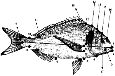
(L)andmarks collected on the sea bream. 1: tip of the premaxillary; 2: tip of the dental; 3: posterior extremity of the premaxillary; 4: insertion of the operculum on the profile; 5, 6, 7, 11, 12, 20, 21: insertion of the fins; 8, 10: points of maximum curvature of the peduncle; 9: posterior extremity of the lateral line. 13, 14, 15, 16: intersection between the profile curve with the equally spaced perpendiculars to the segment connecting landmarks 1 and 9; 18: anterior extremity of the lateral line; 19: posterior extremity of the opercular bone
Landmark configurations were scaled, translated and rotated using the Generalized Least Square method (GLS, software GRF-nD, Slice 1993; available at http://life.bio.sunysb.edu/morph). Landmark configurations were scaled according to centroid size, that is the square root of the sum of the squared distances between each landmark and the specimen’s centroid. A consensus (mean) configuration was computed.
The residuals from the superposition were modelled with the thin-plate spline function. The weight matrix and the uniform components (U1, shearing and U2, stretching, along the major axis of the consensus configuration) were computed.
In order to test for significance the differences in shape between samples, a MANOVA (Wilk’s λ computed with SAS, version 6.01) was computed on non-uniform and uniform shape components.
A canonical variate analysis (SAS, version 6.01) was performed using the non-uniform shape components and a histogram was obtained to visualize the scatter of the two groups along canonical axis 1. The scores of individuals along canonical axis 1 were used as the independent variable in a regression on partial warps (software TpsRegrw, by F.J. Rohlf, version 1.07, available at http://life.bio.sunysb.edu/morph). In this way it was possible to visualize splines (characteristic shapes) relative to each sample.
A scattering of individuals along U1 and U2 was obtained and splines relative to the extreme values of U1 and U2 were visualized.
The relative weight of the uniform and the non-uniform component of shape change was estimated using percentages of variance explained by the regression model (using the canonical variate score as the independent variable) in the case of both shape components (uniform and non-uniform) and for the non-uniform component only. The difference between the two percentages gives an estimate of the weight of the uniform component in determining shape differences. If we denote: u = percentage explained by uniform + non-uniform shape variability; nu = percentage explained by non-uniform shape variability; wnu = relative contribution of non-uniform shape variability in determining the overall shape differences, then, wnu = nu × 100/u
The percentages nu and u are easily computed from the report file of the software TpsRegrw.
Morpho-anatomical descriptors
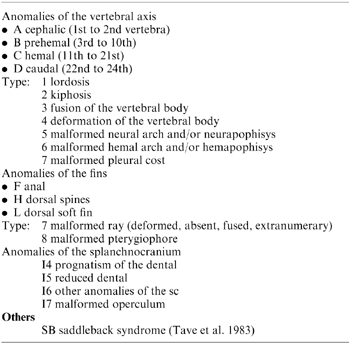
After landmark data collection all individuals were fixed in buffered formaldehyde (10%) and X-rayed (4 min/5 mAmp/ 80 kW). Morpho-anatomical anomalies were then observed and classified according to Table 1. A matrix containing frequency values was obtained and analysed with corresponding analysis. On corresponding axes each individual has a score according to particular patterns of anomalies. On the same plot it is possible to visualize the class of anomalies. Individuals which score closely to particular classes of anomalies are characterized by anomaly cadres defined by such classes.
Geometric morphometrics combined with morpho-anatomical analysis
Individuals scored differently on corresponding axes according to particular anomalies cadres. The scores on each corresponding axis were used as the independent variable in a regression on partial warps. This allowed for the visualization of splines (characteristic shapes) relative to particular patterns of anomalies. Goodall (1991) developed an F-test which gives the significance of the regression model directly in the shape space. Such a test is applied to test whether there is a statistically significant association between shape and scores on all corresponding axes, i.e. morpho-anatomical descriptors. The test is available in the software TpsRegrw.
Results
Geometric morphometrics
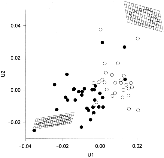
Table 2 shows the results of the manova. The shape differences between the two samples are significant, as also are the differences only in the uniform component. Observing only the uniform component of shape change ( Fig. 2), specimens of the sample SPA (black) show a tendency towards broad profiles (positive values of U1) and a characteristic shearing which result in a prominent frontal region (positive values of U2). Specimens FRA (white) have a more slender body and a streamlined frontal region (negative values of U1 and U2).

)catter of uniform components U1 (shearing) and U2 (stretching and compression). Bottom left spline characterizes negative values of U1 and U2, top right spline, positive values of U1 and U2. Specimens SPA in black, specimens FRA in white
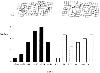
Figure 3 shows the distribution of individuals along canonical axis 1. The two groups are well discriminated. On the top of the histogram, splines relative to the non-uniform component are visualized (localized shape differences).
)istogram of the canonical axis scores. Specimens SPA in black, specimens FRA in white. On the top splines (non-uniform component) relative to extreme values of the canonical axis
Examining the non-uniform component (splines in Fig. 3), three main differences can be emphasized: the first concerns the upper posterior portion of the head region. Relative to the SPA sample, the FRA individuals (right spline) show a rounding of the entire region (defined by landmarks 12, 13, 14, 15, 16 and 1). The profile of the sample does not resemble the typical sea bream profile. In this sample a prominent ventral profile (defined by landmarks 5 and 6) it is also evident. The second main difference concerns the extension of the anal fin base, which is shortened in the FRA sample.
Shape differences are mainly of the non-uniform type which represent 70.04% of between group shape differences.
Morpho-anatomical analysis
Figure 4 shows the distribution of classes of anomalies along corresponding axes 1 and 6 (CA1 and CA6). Only these two axes are significantly correlated with shape variables. The splines reported in the figure are discussed in the next section. Most of the classes of anomalies scatter on the negative portion of CA1; on the positive portion, classes such as prehemal lordosis (B1), malformed ray of the anal fin (F7) and general anomalies of the splanchnocranium (I6) have high loadings. Along CA6, major loadings on the negative portion are those of splanchnocranium anomalies (I6), malformed dorsal soft rays (L7), cephalic, hemal and caudal lordosis (A1, C1, D1).
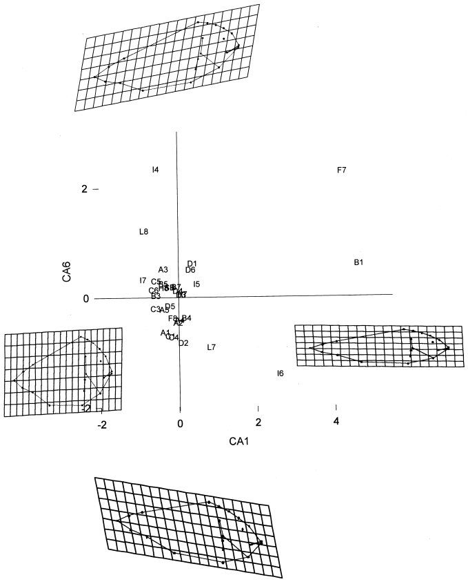
)catters of classes of anomalies on corresponding axes 1 and 6 (CA1, CA6) with associated splines relative to the uniform component only. Left and right splines are relative to extreme values of CA1. The centre top and bottom splines are relative to extreme values of the CA6 axis
Morphometrics combined with morpho-anatomy
Morpho-anatomical data is significantly correlated with shape variables only on corresponding axes 1 (Goodall’s F= 1.49, degrees of freedom (df) = 38, 2166, P = 0.0283) and 6 (Goodall’s F= 1.556, df = 90, 1680, P < = 0.0001).
On corresponding axis 1, only the uniform component is significantly correlated with morpho-anatomical data. On CA6, both components are significantly correlated.
Uniform splines are reported in Fig. 4, non-uniform splines in Fig. 5. In the latter only the splines relative to the extreme values of CA6 are reported, since CA6 is significantly correlated with only non-uniform shape components.
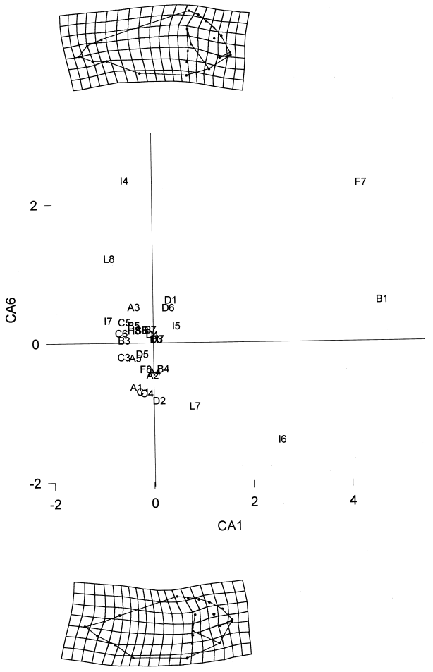
)catter of classes of anomalies as in Fig. 4 with associated splines relative to the non-uniform component only. Scores on CA1 are not significantly correlated with shape variables: splines along this axis are not reported. Top and bottom splines are relative to extreme values of CA6
Most of the anomalies score on the negative portion of CA1: the uniform spline associated with the negative portion of CA1 shows how the typical profile of specimens with high incidence of anomalies is more rounded (left spline, Fig. 4). Low incidence of anomalies is associated with a streamlined profile (right spline, Fig. 4).
A characteristic shearing of the entire ventral part of the body characterizes specimens with splanchnocranium anomalies and different kinds of lordosis (bottom spline, Fig. 4). Minor classes of anomalies scattering on the positive portion of CA6 are associated with a profile with a characteristic shearing of the dorsal portion of the body (top spline, Fig. 4).
Non-uniform splines along CA 6 are reported in Fig. 5. The different kinds of lordosis and splanchnocranium anomalies are associated with a spline (bottom spline, Fig. 5) characterized by a rounded shape of the head region (far from resembling that of a typical sea bream) and a prominent ventral profile. A slight upward bending of the peduncolar region (bottom spline) is associated with caudal kiphosis (D1), while a downward bending (top splines) is associated with caudal lordosis (D2).
On CA1 (mainly differences between high and low incidence of anomalies) the uniform component accounts for 51.3% of the variance explained by the model. On CA6 (where two groups of particular classes of anomalies scatter separately), the uniform component accounts for only 22.9% of the explained variance.
Discussion
As evidenced by geometric morphometrics, S. aurata from different hatcheries is morphologically well discriminated despite common rearing in floating cages over a period of 15 months. The effects of different larval and postlarval rearing conditions are thus persistent. Tightly linked to these conditions is the obtaining of commercial products (wild-like sea bass); the latter may influence the shape to such an extent that stocks by no means resemble the typical profile of the sea bream (sample FRA).
The integration between the morpho-anatomical analyses and geometric morphometrics is appealing: interesting patterns concern the association between the shape of the entire body and the high incidence of anomalies. The profile (linked to swimming and manoeuverability in the transient propulsion of sea bream, Wootton 1990) is streamlined in specimens presenting minor classes of anomalies, while it is rounded in specimens with high anomaly loads. Different kinds of lordosis are associated with a typical shearing of the entire profile: a rounding of the head region, a prominent ventral profile, and a characteristic bending of the caudal region (tightly linked to caudal fin propulsion, i.e. performance, Webb 1984).
The effect of anomalies can be studied at different scales of shape change, uniform and non-uniform, assessing the biological scale at which a certain pattern of anomalies might influence the shape of the fish. In sea bream, high incidences of anomalies can be associated with large scale (uniform) shape changes.
The combined approach evidences how the fish shape witnesses biological underlining patterns such as skeletal characteristics, and it may result in a powerful tool in the evaluation of fish quality. Given the reliability of this method, future research programs could be integrated with genetic characterization in order to link genetic polymorphisms with morphological variability in a broader and more exhaustive framework.


