An optimized autoregressive forecast error generator for wind and load uncertainty study

1 INTRODUCTION

When 20% or more wind generation resources are integrated into the power grid, the wind forecast errors, which can be 70% or more of the grid's generating capacity, will significantly impact the power system generation scheduling process. A market-based generation scheduling process normally includes three planning stages: day ahead (DA), hour ahead (HA), and real time (RT). Based on DA market bids and DA load and wind forecasts, a unit commitment is run to generate hourly power outputs and ancillary services of each committed generation resource. This DA schedule will be adjusted at the HA market based on the HA load, and wind forecasts also use a unit commitment program. Off-line units can be brought online during this process. Intrahour load and wind forecast errors will be balanced by load following, and regulation services are calculated by economic dispatch programs and are provided by online generators that can ramp their outputs up or down within minutes.

If 20% or more of the total load is provided by wind, which is a must-take energy in many markets, the wind generation forecast error can be 14% or more of the total load. Although load forecast errors are normally within 10% of the total load, the online generators normally cannot provide 20% of the total load unless additional units have been committed well ahead of time based on the DA or HA schedules. To make informed, robust decisions on adequate adjustments in generation portfolio and dispatch practices, it is critical to conduct multiple simulations of the generated combinations of wind and load forecast errors to cover the uncertainty range for the standard deviations, the mean values, the autocorrelations and the cross-correlations of the different forecast error time series.

A wind and load forecast error generation algorithm using truncated normal distribution with autocorrelation has been introduced in Loutan et al. 1 and Makarov et al. 2, 3 Because this model was implemented to generate a single forecast error series for wind generation and load, cross-correlation was not considered for different forecasting time frames. An autoregressive moving average model to create wind speed forecast errors that cross-correlated among different wind sites has been developed in Soder.4 Ummels and Meibom et al. 5, 6 implemented this method to produce wind speed forecasts with errors. The wind speed forecasts were then passed through power curves to create generation forecasts. Although these forecasts can be correlated geographically, the model relies on correlating the random series used to calculate each forecast and does not consider the cross-correlation of wind forecast for different time frames.

In this research, we developed a stochastic optimization routine that minimizes the differences between the statistical characteristics of the generated time series and the targeted ones to obtain an optimal set of parameters, which are then in due order of succession used to produce the RT, HA and DA forecasts. The methodology produces random wind and load forecast time series that have the same autocorrelation (of forecasted data points within a forecast series) and cross-correlation (between data points across different forecast series) as the historical real wind and load forecast data.

This paper is organized as follows: Section 2 presents the load and wind statistics derived from the real data sets, and Section 3 introduces the algorithm of the stochastic optimization-based first-order autoregressive forecast error generator. The results are discussed in Section 4, and conclusions are presented in Section 5.

2 LOAD AND WIND FORECAST CHARACTERISTICS

To be integrated with unit commitment and economic dispatch processes, wind generation and load are assumed to be forecasted in three different time frames: DA, HA and RT. The DA forecast is produced for the 24 one-hour intervals of the following day. The HA forecast is updated each hour, and the RT forecast is updated every 5 min.

2.1 Wind forecast statistics

The forecast error, ε_w, is normalized to the wind plant capacity, C_w, as follows:

(1)

where G_w is the actual wind generation. Figure 1 shows a few plots of normalized wind forecasts and wind forecast errors of an example wind site from the California Independent System Operator (CAISO) data. Note that the wind forecast, F_w, is more accurate when forecasts are made closer to real time.

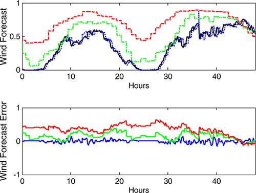
Statistical characteristics of the forecast errors were calculated using actual historical forecast errors from the CAISO system. Table 1 summarizes the wind forecast statistics obtained from CAISO-controlled wind plants. The autocorrelations of t to t−1 time interval for the RT, HA and DA forecasts and the cross-correlations of the HA with RT and the DA with the HA forecast error time series are shown in Table 1. The wind forecast error distributions (FEDs) are shown in Figure 2.

Table 1. Wind forecast error statistics

	Standard deviation (%)	Mean values (%)	Autocorrelation (t, t−1) (%)	Cross-correlation (%)
RT	9.69	1.36	97.01
HA	9.62	2.06	82.82	41.69
DA	13.58	0.08	93.14	66.75

These three wind forecast error time series have the following characteristics:

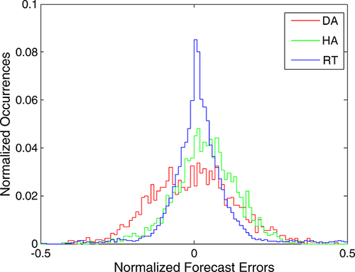
• The error distributions are ‘bell-shaped’ and in this regard are similar to Gaussian, although they do not strictly match. The RT errors tend to have many very small errors and a few large errors. The DA and HA errors tend to be asymmetrical.
• There is significant autocorrelation between the t and t−1 values.
• The HA and RT as well as the DA and HA forecast error time series are cross-correlated.
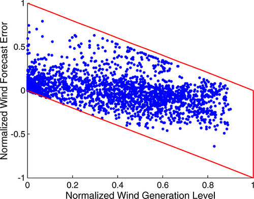
• The forecast errors are constrained by the available wind generation range as shown in Figure 3. A reasonable forecast for wind generation must stay between zero and the capacity of the wind plant. The red lines trace the bounds of the forecast error. The forecast errors tend to be positive at lower generation levels and more negative at higher production levels.>

2.2 Load Statistics

The forecast error, ε_L, is normalized to the load output at the time L_t as follows:

(2)

Historical forecast data from the CAISO system were used to develop the statistics of the load forecast error. Similar to the wind forecast errors, the autocorrelation between N and N −1 time intervals and cross-correlation of the HA with the RT and the DA with the HA load forecast time series are also significant, particularly with respect to the DA and HA forecasts errors. Table 2 summarizes the statistics characterizing the load forecast errors.

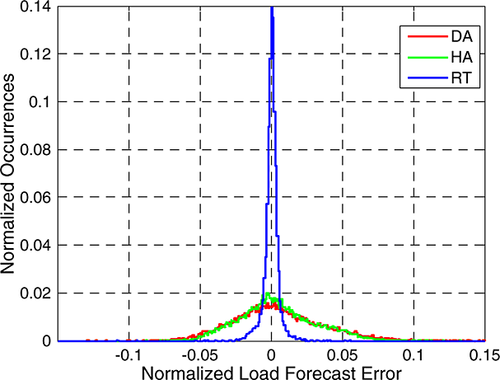
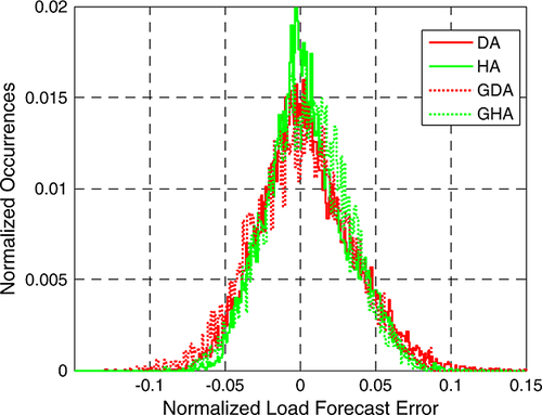
The overall shape of the load FEDs is similar to the wind FEDs (Figure 4). The RT forecast errors are very highly concentrated near zero, with a few high error occurrences. The DA and HA errors have similar shapes, with the DA errors having a larger variance.

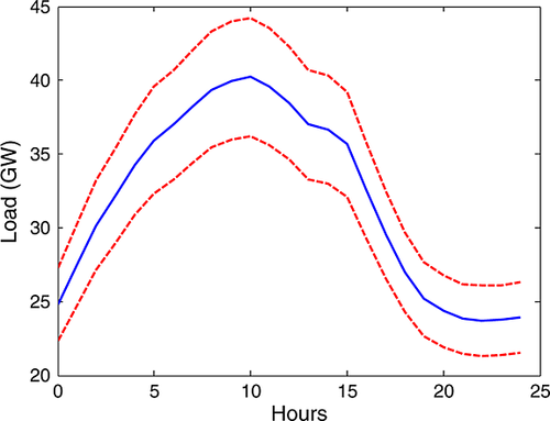
The load forecast errors do not have the same ‘natural’ bounds as the wind forecast errors, which are bounded by the wind farm capacity. However, load forecast errors can be bounded using a fixed percentage, for example, ±15%, which represents the maximum error to vary with the load. This is consistent with the observed trends. High load periods tend to have a larger forecast error because of the sensitivity of load forecasts to temperature forecasts. Figure 5 shows how the error bounds change on a typical day. The blue line is a typical daily load profile, and the red dashed lines illustrate the bounds placed on the forecast errors.

Table 2. Load forecast error statistics

	Standard deviation (%)	Mean (%)	Autocorrelation (%)	Cross-correlation (%)
RT	0.53	0.02	56.16
HA	2.66	0.39	78.22	11.86
DA	3.12	0.41	84.52	82.81

3 METHODOLOGY TO SIMULATE FORECAST ERRORS

3.1 Mathematical model

Our objective was to develop a random forecast error generator that produces multiple time series for the RT, HA and DA wind and load forecast errors. For each of these time series, the standard deviation, the mean value and the autocorrelation coefficient between the t and t−1 points must match those derived from the historical forecasts. Between the RT and the HA as well as the HA and DA time series, the cross-correlation coefficients must also match. The following first-order autoregressive model can be used:

(3)

where X is the time series to be generated; Y is the exogenous time series with zero mean to be cross-correlated with X; e is the Gaussian random series with zero mean and autocorrelation and specified standard deviation; a, b, c and d are the coefficients; t is a time interval and N is the number of time intervals.

If we assume that the mean value of X is zero, then the standard deviation σ_X, cross-correlation C_{X, Y} and the autocorrelation can be expressed by

(4)

(5)

(6)

Let the error time series e have the same standard deviation as the to-be-generated time series X. With some simplification, we have

(7)

(8)

(9)

Note that the e and Y series are not cross-correlated; therefore, the cross-correlation coefficient C_e, Y is zero. These forms of the equations could not be solved simultaneously to determine the optimal values of the parameters a, b and c because the correlations C_X, e between the X and e time series are unknown. Therefore, to find the appropriate values of the unknown parameters a, b and c, an optimization routine was used. The optimization routine was set up to minimize a non-linear objective function that measured the difference between the desired statistics and the calculated statistics; the objective function takes the form

(10)

where X is the time series to be generated; σ_g is the target standard deviation of X; is the target mean of X; is the target autocorrelation between the t and t−1 points of X; is the target cross-correlation between the X and Y time series; σ_e is the standard deviation of e and k₁, k₂, k₃ and k₄ are the weighting factors of the objective function.

The optimization process is an unconstrained non-linear optimization problem and is solved with the Nelder–Mead algorithm using the MATLAB (The MathWorks, Inc. headquarters in Natick, Massachusetts) optimization toolbox.7

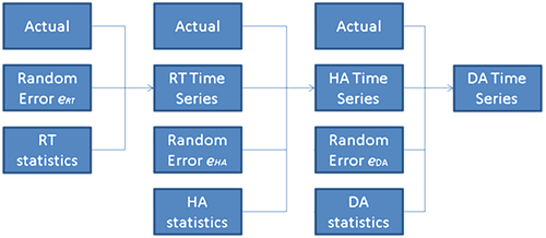
The methodology to generate the correlated forecast errors based on an actual time series is a sequential process. As shown in Figure 6, the RT forecast errors are generated first. Because the RT forecast error is generated independently, b_RT = 0. The HA forecast error is generated next, followed by the DA forecast error time series.

The calculations for the RT, HA and DA series are as follows:

(11)

4 RESULTS

The methodology was used for expected load and wind production levels in 2012 to produce 100 DA, HA and RT wind and load forecast error time series. Wind forecasts are developed for five major wind areas within California. Load forecasts are developed for the three investor-owned utilities in the state. In all cases, the model produced forecast error time series that matched the autocorrelation, the standard deviation and the mean of the existing forecast error statistics. The cross-correlations between the generated time series matched well except for the one between the RT and HA load forecast errors. This is because this correlation is rather weak and the optimization routine was weighted to put more priority on matching the standard deviation.

4.1 Wind forecast error generation

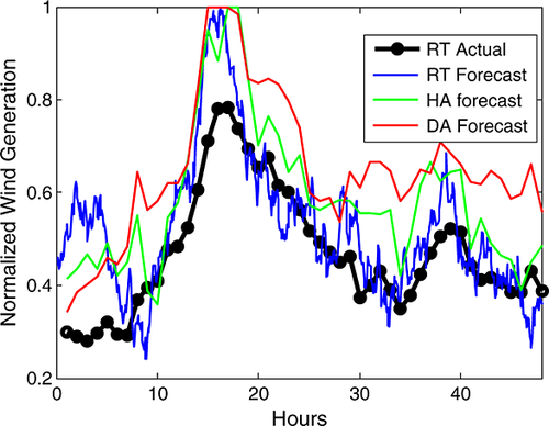
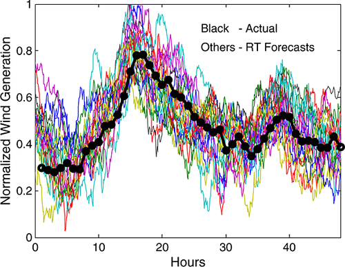
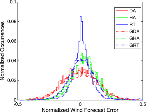
One hundred realizations of wind forecast errors are generated for a given estimation of the 2012 wind generation profile. The 100 realizations represent 100 of the possible RT, HA and DA forecasts for the given wind profile. An example of the actual and RT, HA and DA forecasted wind is shown in Figure 7. Figure 8 shows a plot with the actual wind generation curve and the 20 runs of RT forecasts. In this figure, the forecasts form a range about the actual profile. The generated forecast time series cover the space within which the RT forecasts can fall. The FEDs of the modeled error series are shown in Figure 9. Compared with Figure 2, the DA and HA FEDs are similar, although the modeled RT FED has many more mid-range errors than what occurred in the observed forecast data.

4.2 Load forecast error generation

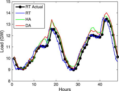
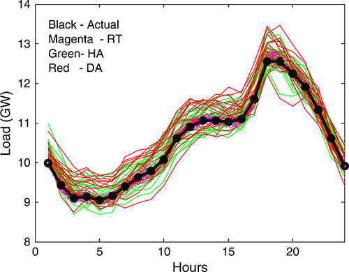
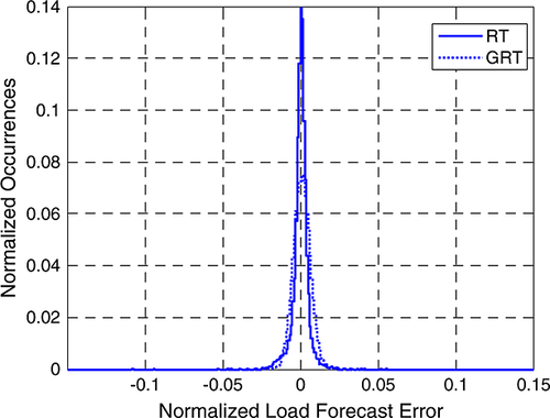
The load forecasts are generated similarly to the wind forecast errors. Figures 10 and 11 compare an example of some DA forecasts with the actual profile. The forecasts follow the basic shape of the profile and provide a range of variability around the profile. The FEDs of the modeled forecast errors (see Figures 12 and 13) are similar to those of the observed wind forecast errors.

5 CONCLUSIONS

This paper presents a stochastic optimization-based first-order autoregressive forecast error generator. The methodology aims at producing random wind and load forecast time series that match the following statistics of historical forecast data sets: the means, the standard deviations, the autocorrelations and the cross-correlations between RT, HA and DA forecasts. A stochastic optimization routine weights the differences between the target statistics and those of the generated time series to obtain the optimal parameters that produce the forecasts.

Results show that the methodology produces random series with the desired statistics. The error generator has been used in wind integration studies to provide wind and load forecasts for stochastic unit commitment. This method, although implemented as the first-order regressive random forecast error generator, can be extended to higher orders. However, there is a trade-off on weighting different optimization objectives. Our study shows that for RT load forecast, matching the HA forecast standard deviation can force the cross-correlation between the HA and RT forecasts to deviate from the target values.

Our future studies will focus on reflecting the diurnal and seasonal differences of the wind and load statistics and implementing them in the random forecast generator.