Time series modelling of power output for large-scale wind fleets

1 INTRODUCTION

A great deal of research has been devoted to the development of time series models for the wind speed at a fixed location.1-10 These models, which are generally based on autoregressive (AR), autoregressive moving average, Markov chains or spectral methods, have been developed either to assist with short-term wind speed prediction or for use in power system simulations. We are concerned here with the latter application. Such models are hard to extrapolate to a large fleet because a single wind speed can only pertain to a single location, whereas a country-scale power system may contain hundreds of wind farms distributed over hundreds or thousands of kilometres. One solution would be to use a multivariate model such as a vector autoregressive one,11, 12 but these models can run into calibration difficulties because of the very large number of parameters that are required if many sites are to be represented. Klöckl and Papaefthymiou12 described this problem and some techniques that could be used to mitigate it.

A simpler approach is to model the wind power instead of the wind speeds, as Papaefthymiou and Klöckl13 did for a single location using a Markov chain Monte Carlo technique. This technique could be equally well applied to aggregated wind output for a large fleet, for which some long-term and transitional statistical properties have recently been analysed by Louie.14, 15

We have developed a wind model for our single-bus power system operation simulations, for generating synthetic wind power samples and also for supplying statistical information to the stochastic scheduling algorithm. It is a low-order, univariate AR model that can be fitted to historic, aggregated, time-averaged wind power output data from a geographically diverse fleet of wind farms, without explicitly modelling the wind speeds. The objectives of the model are: to reproduce the same long-term (asymptotic) distribution of power outputs as the historic data, to reproduce the same diurnal variation of the average power output, and to reproduce the same average power output changes over timescales up to around 4 h, which is a typical start-up time assumed for combined cycle gas turbines and therefore represents a crucial lead time for scheduling thermal reserve plant.

The technical development of this paper is divided into three sections. In the next section, we develop the methodology behind our model. Section 3 introduces three data sets to which we have fitted our model, from New Zealand, Denmark and Germany. Results from the calibration are discussed in Section 4. These include an assessment of the fit to some transitional properties to which the model is not explicitly calibrated.

2 METHODOLOGY

Gaussian linear time series models23 are straightforward to fit historic time series data and have well-understood asymptotic and transitional properties. However, they cannot be used directly to generate samples of wind power because real wind processes are non-Gaussian and have diurnal and seasonal components. Our approach is to use a Gaussian linear AR process as the underlying driver but transform it by adding on a periodic diurnal term and then, by using a memoryless non-linear function, transform the process into one with the required asymptotic distribution. Seasonal variations are accounted for by dividing the year into a small number of seasons and fitting separate models to each season.

The underlying driver of the model is an AR(p) process, which is driven by independent N(0,1) variables ε_k:

(1)

We scale the parameters so as to normalize the asymptotically stationary distribution of X_k to N(0,1). This allows us to fit the model in two stages. First, we find the transformation function and the diurnal term that reproduce the historic overall power output distribution and diurnal variation of the mean. Second, we find the AR parameters that provide the best fit to the short-term dynamics.

The diurnal variation is introduced by an additive term μ_k with a period of N_T, the number of time steps per day (typically 24 or 48):

(2)

which means that the cumulative distribution function (CDF) of is

(3)

where N(x) is the standard cumulative Gaussian distribution.

Most wind speed model-fitting studies, such as that of Brown et al.,2 use a power transformation to convert the (approximately Weibull) wind speeds to an approximately Gaussian variable. This class of transformations is not suitable if, as here, the historic input takes the form of wind power rather than wind speed. The beta distribution has been suggested by Louie15 for aggregated wind output. An alternative, implemented here and in a study by Klöckl and Papaefthymiou,12 is to estimate the distribution non-parametrically by direct observation of the historic data. We first estimate the CDF of the historic power output values P_k using Parzen windowing and then choose a transformation function W(·) that is guaranteed to generate values with the same CDF as P_k given that its argument is distributed like . We can achieve this by writing

(4)

where C(x) is the CDF of P_k.

We stipulate a diurnal variation such that the expected power output at discrete time-of-day i(= k mod N_T) is which means that since X_k ∼ N(0,1),

(5)

where ϕ(x) is the standard Gaussian probability density function.

The choice of the transformation function W(·) and the vector (μ_i) can therefore give rise to any desired overall distribution of power output as well as the diurnal variation of its expectation. This is a more parsimonious formulation than that in Klöckl and Papaefthymiou,12 which requires separate transformation functions for each time of the day but is able to represent the diurnal variation of the distribution more fully. The determination of W(·) and μ_i from C(·) and requires an iterative method because equations 3-5 represent a set of coupled non-linear equations. Details of a simple solution method are given below.

First, we note that the equations are overdetermined because an arbitrary constant can be added to all the μ_i without affecting the solution. If is inconsistent with C(·), then there will be no solution, whereas if they are consistent, then there are infinitely many solutions, and we can arbitrarily add the following constraint:

(6)

Having thus determined the function W(·) and the vector (μ_i) to satisfy the required long-term statistics of the power output, our next task is to reproduce the desired transitional statistics. This is achieved by manipulating the parameters of the AR model [equation 1] while maintaining the requirement that its asymptotic distribution is N(0,1). One way to fit the data is to transform the historic power output into values of X using

(7)

and to obtain the AR parameters (φ_n) using standard fitting methods such as the Yule–Walker equations,23 which in the case of an AR(1) model reduces to

(8)

If X follows an AR(1) process, then its asymptotic variance is

(9)

and since we have designed μ_i and W(X′) to produce the correct long-term statistics when X_k ∼ N(0,1), it follows that

(10)

If X follows an AR(2) process

(11)

then the Yule–Walker equations can be used to derive φ₁ and φ₂ as the solution to the linear system

(12)

where c_i = E[X_kX_k − i], and σ then follows from the formula derived by Box and Jenkins23

(13)

and the requirement that , as before.

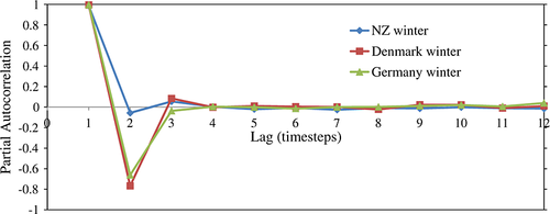
The appropriate order of the AR model can only be determined by careful analysis of the underlying data on a case-by-case basis. If there is no trending in the data (i.e. no significant autocorrelation between successive increments in the X domain), then a first-order model will suffice. However, any smoothing effect from the aggregation of large numbers of wind farms will manifest itself in trending behaviour, so that a second-order (or higher) model may be necessary. (The smoothing effect will be further enhanced if the time series data consist of time-averaged values, as in the case studies documented here.) The Akaike information criterion, autocorrelation function and partial autocorrelation function (PACF) can be used to help the analyst choose appropriate model orders to provide the best fit to the X domain values. We used PACFs for each data set to help determine appropriate model orders and confirmed our choice by observing the goodness of fit of the volatility in the P domain in each case over a range of time horizons.

3 CASE STUDIES

These three cases provided contrasting challenges for the model: a small number of very dispersed sites with a high capacity factor and half-hourly resolution (New Zealand), a large number of sites in a much smaller region and hourly resolution (Denmark), and a very large installation with hourly resolution (Germany).

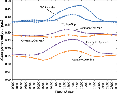
All cases show significant seasonal and diurnal periodicity, indicating that a multiseasonal model with diurnal adjustment is necessary (Figure 1). For the Danish and German cases, capacity factors were considerably higher in winter than in summer. In the New Zealand case, there was no significant difference in the average power output, but there was significantly more diurnal variation in summer than in winter. We fitted separate models to four seasons in the Danish and German cases: spring (March–May), summer (June–August), autumn (September–November) and winter (December–February). For the New Zealand case, we used just two seasons: summer (October–March) and winter (April–September).

A model should be calibrated and validated using separate sections of the data, if it is to have credible predictive ability. This was not practical for the New Zealand case because of the rather short available data set. For the Danish and German cases, we calibrated the models to the first two-thirds of the data only, so that the last third could be used as an independent validation data set. However, in all cases, we present histograms for each sample year in order to give an idea of the likely degree of interannual variability of their respective wind regimes.

4 MODELLING PRACTICALITIES AND RESULTS

The target power output CDFs C(P) were estimated by Parzen windowing, using a Gaussian kernel with a standard deviation of 0.02 p.u. in each case. The target average outputs (), representing the expected power output for each time step during the day, were also measured from the data (Figure 1). The values were slightly noisy, so we smoothed them by replacing each element of with a moving average of itself, the previous value and the following one. This prevented the model from generating partially predictable jumps at the same time each day. We then used the iterative technique described in Section 2 to find the transformation function W(·) and the vector (μ_i) that would provide an exact match to the measured long-term distribution and diurnal variation. Figure 2 shows two examples of the transformation function. Its sigmoid shape ensures that the near-Gaussian variable X′ is transformed into one with the correct power output distribution, that is bounded between zero and the maximum allowable value.

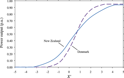
Next, we transformed the historic power output data (P_k) to normalized values (X_k) and calculated the PACFs to inform the choice of model order. Figure 3 shows the first 12 elements of the PACFs for the winter data sets of each region. It suggests that, although first-order model is adequate for the New Zealand data, second-order ones are necessary in the case of Denmark and Germany. This was confirmed by fitting AR models of various orders and examining the fit of volatilities of the transformed (power output) process for horizons up to 8 h. Table 1 shows the fitted AR parameters. When fitting AR models with the Yule–Walker equations, we excluded values of P corresponding to flat regions of the W curve (Figure 2), as X is undefined in these regions. All cases show the parameters calculated from the Yule–Walker equations, with the exception of the New Zealand summer data for which the volatility parameter σ was lowered slightly (and φ₁ increased) in order to improve the fit to the dynamics of the transformed (power output) process. The fact that some manual adjustment was required demonstrates that the best fit in the X domain does not necessarily lead to the best fit in the P domain because of the non-linear transformation that links the two domains. For example, portions of the time series corresponding to regions of the W curve that are nearly flat (e.g. where the power output is close to zero) may give rise to residuals with different properties from those that arise from other parts of the curve. However, failure to model these differences will not necessarily compromise the performance of the model in the P domain, since large changes in X only cause small changes in P in these regions.

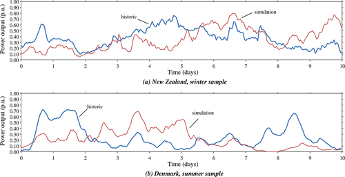
Two 10 day samples of the time series are shown in Figure 4, for historic and simulated cases in New Zealand and Denmark. The much noisier signal for the New Zealand case, with far fewer sites, can be easily identified. The diurnal variations for the Danish summer case, peaking just after midday, are clearly visible in both historic and simulated cases. The simulated power output samples are optically very similar to the historic ones, but we tested the goodness of fit of the model in a more quantitative fashion, by comparing the dynamics of the power output time series for the historic and simulated cases. It should be noted that, although the model has enough degrees of freedom to allow an exact calibration to the long-term distribution and diurnal variation, there is only one free parameter in an AR(1) model and two in an AR(2) model, to fit all the desired transitional properties. The following sections examine the performance of the model with regard to the power output distribution, the volatility over a range of time horizons, the occurrence of large changes, the relationship of expected power output change with the power output level and the occurrence of periods of low output (calms).

4.1 Power output distribution

The model is explicitly fitted to the long-term (asymptotic) power output distribution of the calibration data set. In this section, we examine its performance with regard to each year of historic data from both calibration and validation data sets.

Figure 5(a)(i),(b)(i),(c)(i) shows power output histograms for each year of the New Zealand, Denmark and Germany data sets, respectively. The diamond and square markers show calibration and validation data, respectively. It can be seen that there is a fair amount of interannual variation although the overall shapes are broadly similar in all years.

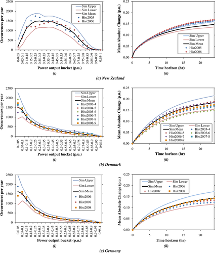
Some interannual variability is also seen in simulation despite the model's fixed parameters because different samples of the random number drivers are used for different simulation years. The black line shows average values from 1000 annual simulations, whereas the upper (blue) and lower (pink) curves show, for each histogram bucket, the 97.5th and 2.5th percentile values from the simulations, respectively. Hence, if the model correctly models the interannual variability, we expect 95% of historic data to lie within these curves. It can be seen that both calibration and validation data sets are generally within the simulated range, indicating that the interannual variation in simulation is generally of the correct order of magnitude—although the quantity of validation data is insufficient to assess this precisely. Two possible exceptions are the rather calm year 3 (green diamonds) and the rather windy year 4 (purple diamonds) of the Danish calibration data; in both cases, simulation produces such extreme capacity factors for 1 year in every 15 years or so.

4.3 Distribution of changes in power output

Since reproducing the expected power output changes over a range of timescales, the model must also reproduce the correct distribution of these changes. Of particular concern is the incidence of sudden large changes, particularly downward ones, because a system that is operated with inadequate reserves is vulnerable to involuntary load shedding if the wind feed-in drops too quickly. We looked at the performance of the model with regard to the distribution of power output changes over 1 and 4 h. Figure 6 shows histograms of absolute power output changes over these horizons for each region, for each historic sample year and for the range of simulated values. Occurrence rates of the full range of power output changes, and their interannual variability, are generally well represented by the model, although there is a slight tendency to under-represent the occurrence of the most extreme changes (occurring up to a few times per year) in the Danish case. The outlier in the Danish 4 h 0.60–0.65 bucket is due to the violent windstorm that struck Denmark on 8 January 2005, causing the majority of the Danish wind fleet to cut out over a short period. The lack of an explicit representation of turbine cut-out prevents the model from reproducing these rare ramping phenomena.

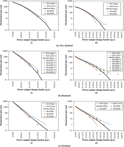
The log-linear appearance of some of the power output change histograms is indicative of a Laplace distribution, as has been noted by several other authors15, 26 over a range of timescales and for regions of various sizes. The New Zealand data, which represent a 2000 km region, seem to be somewhat sub-Laplace, which should be expected for very large regions because of the central limit theorem, as noted by Louie.14

4.4 Relationship between power output level and power output changes

The previous sections demonstrate that our aggregated wind fleet model reproduces the long-term distribution, the diurnal variation and the distribution of power output changes over timescales up to a few hours, for the three cases examined in this work. In this section and the next, we examine some other transitional statistics to which our model is not explicitly calibrated. If the model represents the physics of the system at some level, then we might hope that these statistics could nevertheless be captured, at least qualitatively.

The volatility of power output for a single wind turbine is a function of the power output level itself. This is partly due to the lower wind speed volatility at low wind speed levels, but more importantly, the power output volatility is affected by the non-linear nature of the wind turbine power curve, which maps wind speed to wind power. At very low wind speeds, the power output is zero, so that the power output volatility is also zero. At high wind speeds between about 12 and 25 m s⁻¹, when the turbine curve has reached saturation, the power output volatility is also theoretically zero. At moderate wind speeds, small changes in wind speed can have a large effect on the power output, so that the volatility is high. At very high wind speeds (typically around 25 m s⁻¹), the turbine cuts out to prevent damage, resulting in near-instantaneous jumps between maximum output and zero and extreme volatility of power output.

A similar behaviour is to be expected when many turbines are aggregated because of the correlation between wind speeds at the different sites, although the volatility will be reduced by aggregation, particularly at very high outputs because not all turbines will cut out at the same time if they are distributed over a wide area.

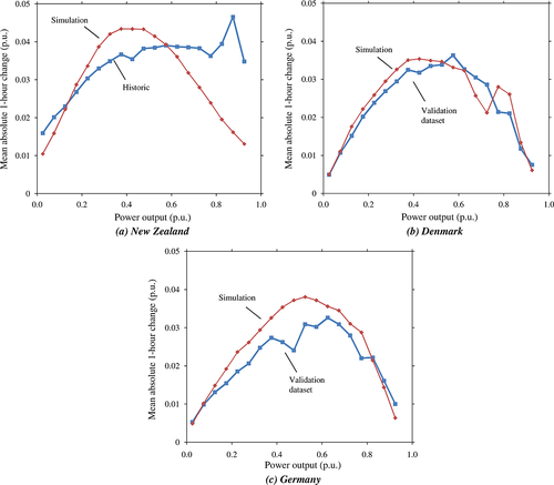
It may be important to reproduce this behaviour in a power system simulation because the amount of thermal plant online, and hence the maximum amount of available spinning reserve, will decrease as the wind power production increases. We expect our model to reproduce some of the behaviour. In a sense, the diurnally shifted AR variable, X^′, is a measure of the overall ‘windiness’ of the region, and the transformation function W(·) (Figure 2) is a ‘power curve’ for the aggregated wind fleet. Unlike a real turbine power curve, however, our aggregated power curve does not have an explicit cut-out, so that we might expect the model to underpredict the volatility at very high power outputs.

Figure 7 shows the mean absolute change over a 60 min time horizon for the three cases. In New Zealand [Figure 7(a)], the small number of highly dispersed sites leads to a high overall volatility at high wind levels as a result of turbine cut-out; as there are only 15 sites, cut-out at a single site would lead to an aggregate power output drop of nearly 0.07 p.u. As expected, the model fails to reproduce this and exhibits considerably lower volatility than the historic data at high power levels. However, for the Danish [Figure 7(b)] and German [Figure 7(c)] cases, which represent hundreds of sites, the model provides a good match to the historic properties, with peak volatility occurring at around 0.60 p.u., although the model volatility is generally higher than the historic data in the German case.

5 CONCLUSIONS

This paper has shown that a time series of hourly or half-hourly, time-averaged power outputs for large-scale wind fleets can be readily modelled using a low-order AR model, in conjunction with a diurnal adjustment and non-linear transformation function. The long-term distribution of the power output, as well as the diurnal variation of mean power output, can be represented exactly by using a straightforward calibration procedure, and the interannual variability of the distribution in simulated data sets is of the same order of magnitude as for the historic ones analysed in this work.

Another important statistic, when integrating wind with thermal plant that is constrained by start-up times or ramping limits, is the behaviour of power output changes up to a few hours. A first-order model (New Zealand) or a second-order one (Denmark, Germany) can capture the average change over time horizons up to around 8 h. The need for a second-order model implies that a Markov chain representation of an aggregated wind fleet would require two state variables, i.e. the current wind power and the wind power at the previous hour, so that a large transition matrix would be required to cover the entire state space with a fine granularity.

The distribution of changes is close to a Laplace distribution, as has been noted by several other authors working with data sets from around the world. Data sets from very large regions (e.g. New Zealand) have somewhat sub-Laplace tails because of the effects of the central limit theorem. Despite being based on a Gaussian time series, the model provides similarly fat tails in the distribution of changes because of the non-linearity of the transformation function, which makes the short-term volatility a function of the current wind output level. For large-scale fleets with hundreds of sites, the historic data show a similar relationship, with a peak volatility at around 0.6 p.u. and much lower levels at very high or very low outputs. With fewer sites, the lack of an explicit model of turbine cut-out leads to an underestimate of the volatility at high outputs. For the same reason, the model does not reproduce large rapid changes in aggregate output because of wide-scale turbine cut-out during storms that affect a high proportion of the fleet.

The model provides an acceptable representation of the distribution of periods of low output (calms) from 2 h to 7 days in length. This statistic may be important if the wind fleet is to be integrated with medium-term storage or demand-side measures. The frequency of very short calms is underestimated by 15–30% in the cases considered here, and the frequency of very long calms, occurring less than once per year, is also underestimated in the Danish case because synoptic effects are not explicitly modelled.

The supply and demand of many power systems is dependent on temperature as well as wind because of heat-led combined heat and power plants and electrical heating, for example. Since wind and temperature are not independent variables, care should be taken when using an independent wind model in simulations of temperature-dependent systems.

One limitation of the model lies in its univariate nature. Recent wind integration studies, such as TradeWind,21 focus on the use of power transfers between interconnected country-sized European regions to minimize the overall impact of wind intermittency. Since these power flows are constrained by the limited transmission capacity between regions, multiregion studies need to model the wind feed-in separately for each region. In theory, our model could be extended to a multivariate version in order to account for the correlations between regions. Care would be needed to ensure that the long-term joint distribution is adequately represented, as well as the correlations between power output changes in different regions.