Reducing coherent filtering artefacts in time-domain operational modal analysis
Funding information: Alan Turing Institute, Grant/Award Number: Turing Fellowship; Engineering and Physical Sciences Research Council, Grant/Award Number: EP/R513209/1
Abstract
Signals collected for modal analysis are often filtered in order to reduce sensor noise, out-of-band oscillations, or for dealing with closely-spaced modes. This filtering introduces filtering artefacts into the data due to the non-ideal filter response and is well understood for impulse excitation. However, for ambient vibration data filtering, artefacts become superimposed, preventing their visual identification, and will corrupt the correlation function of the data used in time-domain operational modal analysis (OMA) techniques such as covariance-driven stochastic subspace identification and the random decrement technique. This corruption leads to inaccurate, misleading, biased or spurious frequency and damping estimates, with the inaccuracy increasing for systems with higher damping or lower signal-to-noise ratios. Counter-intuitively, the error in damping estimates is as large for modes with natural frequencies far from the filter cutoff frequency as for modes which are close to the cutoff frequency. In this paper, an alternative to filtering for time-domain OMA, trimming of the correlation of noise from unfiltered correlation functions, is introduced and tested using 10,000 numerically generated ambient vibration data sets. It has been shown that this technique reduces the mean absolute error in the frequency estimates by over 200% and the mean absolute error in the damping estimates by over 400%. Additionally, a new technique which incorporates fitting of filtering artefacts as part of the modal analysis is introduced for where filtering of ambient vibration data is unavoidable and is demonstrated using real-world acceleration data collected from a two-way spanning concrete slab subject to footfall excitation.
1 INTRODUCTION
Due to the size and complexity of many civil engineering structures, it is not possible to measure their dynamic properties using conventional forced vibration analysis. Operational modal analysis (OMA), whereby the ambient vibrations induced in a structure during everyday use form the excitation force, has therefore become an essential tool for the modern structural engineer.1-5 It is common practice for ambient vibration data collected for use in OMA to be filtered prior to analysis6 in order to remove sensor noise, interfering signals such as the mains electricity frequency, vibrations caused by heating and ventilation systems, modal oscillations outside of the frequency range of interest, or to allow analysis of closely-spaced modes.5, 7-15 However, a number of researchers have noted that the results obtained through time-domain OMA techniques are sensitive to the filtering of the data.16-21 Aquino and Tamura16 noted that the filtering of ambient vibration data prior to analysis with the random decrement technique led to changes in the damping ratios; a key parameter in the design of civil structures which affects how long unwanted oscillations may persist, the amplitude which oscillations may reach, and the likelihood of resonance being induced in the system. Other observations on the impact of filtering on the random decrement technique include earlier work by Tamura17 and the original observations made by Cole18 during the development of the technique. For both covariance-driven and reference-based stochastic subspace identification methods, filtering of the data leads to the introduction of spurious modes as noted by Reynders et al19 and Peeters and de Roeck.20, 21 This complicates the identification of structural modes within the stability diagram.20, 21 While the impact of filtering artefacts on experimental modal analysis22-24 and on signal processing for system identification25, 26 is well understood, the impact of filtering on ambient vibration data analysis, where it is the coherence of filtering artefacts within the data which distorts modal parameter estimates, has not previously been addressed.
In this paper, it is demonstrated that filtering artefacts associated with Gibbs phenomena are the cause of these variations in estimates of modal properties and that the impact of filtering on damping estimates may be in the order of hundreds of per cent of the true damping value.
Counter-intuitively, the corruption of damping estimates is largely independent of how far the filter cutoff is from the frequency of the mode. Instead, the magnitude of the corruption of damping estimates is driven by the ratio between the amplitude of the filtering artefacts and the amplitude of the modal component of the time-domain signal to be fitted, a ratio which is dependant on both the signal-to-noise ratio of the data, and the relative amplitudes of different modes of vibration.
The paper is organised as follows. The cause of filtering artefacts is presented, and their impact on two common time-domain OMA methods, the random decrement technique and covariance-driven stochastic subspace identification, is demonstrated using numerically generated data. A new method is demonstrated for the identification of filtering artefacts using the random decrement technique. Using this technique, it is shown that the use of a filtered data set within the vector random decrement technique27 may lead to filtering artefacts appearing in unfiltered data sets due to the coherence of segments across data channels. A new technique, based on ‘trimming’ the noise component/filtering artefacts from the unfiltered time-domain correlation/free-response signals is introduced. Using numerically generated data from a 2 degree-of-freedom (DOF) system, it is shown that this technique drastically reduces the errors in both frequency and damping estimates when compared to the untrimmed signals or the filtered signals. Using the numerically generated data, it is shown that the impacts of filtering artefacts are more acute for systems with higher damping and for systems with lower signal-to-noise ratios. Furthermore, it is shown that filtering artefacts introduce significant errors in the damping ratio even when the filter cutoff frequency is far from the natural frequency of the mode of vibration. Finally, a new method for removing the effects of filtering artefacts through the use of an indicative noise profile in the time-domain OMA is presented for use when filtering of the ambient vibration data is unavoidable. This procedure is demonstrated using real-world data collected from a two-way spanning concrete slab.
- Demonstrating the link between the biassing of modal estimates introduced by filtering and the characteristics of impulse response functions and quantifying their impact on modal estimates using simulated and real-world data.
- Providing practical guidance on how to limit the bias introduced by filtering in OMA.
- Introducing a practical alternative to filtering for improving time-domain modal estimates through trimming of the autocorrelation of the noise from unfiltered time-domain correlation/free-response signals.
- Providing a method through which filtering artefacts may be removed or minimised using an indicative noise profile and fitting of the filtering artefacts as part of the modal analysis for use where filtering of the data is unavoidable.
2 BACKGROUND AND THEORETICAL BASIS
2.1 Filtering artefacts
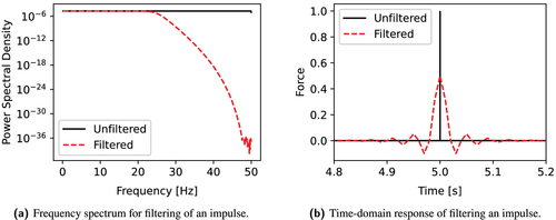
As shown by Equation 2, the duration of the ‘ringing’, here called the length of a single filter artefact oscillation, is dependant on the frequency cutoff of the filter, , with the amplitude of the filter artefact oscillations related to the filter order (the sharpness of the frequency roll-off), the type of filter used, and amplitude of the initial discontinuity.31
A factor which complicates the initial identification of filtering artefacts in ambient vibration data is that filtering of noise leads to a smoothing effect of the underlying signals, making visual distinction between filtering artefacts and real dynamic oscillations in the signals more difficult.
2.2 Artificial data generation
For the purpose of demonstrating the origin and impact of filtering artefacts in Sections 2.3 and 2.4, , and . This gives natural frequencies and damping for the 2DOF system of 5.69 Hz with 1.4% of critical damping and 2.19 Hz with 3.64% of critical damping. The data used in Sections 2.3 and 2.4, referred to as the 2DOF example data, consisted of 60 min of displacement data for each DOF, generated at 100 Hz using the Newmark-beta method, resulting in 360,000 samples of data for each DOF. The 2DOF system was excited with a Gaussian white-noise process independently at both DOFs with a mean value of 0 N and a standard deviation of 20 N.
The Newmark-Beta method does not attenuate the instantaneous force response of a system as a real structure does, resulting in instantaneous changes in the acceleration and velocity in the generated data which are not present in data collected from real-world systems. Therefore, displacement data were used to avoid the generation of the component of the autocorrelation function associated with the input force.33
Additive white noise was independently added to the displacement data from both DOFs to achieve a modal signal-to-noise ratio (SNR1) of 3. The modal SNR of the data is here defined as the ratio between the amplitude of the frequency spectrum of the uncorrupted data and the noise data, averaged across both natural frequencies of the system and across both of the DOFs. Additive white noise is used to demonstrate the impact of filtering artefacts on time-domain OMA, with non-white noise addressed in Section 5.
2.2.1 Filter parameters
Within this paper, the Butterworth filter with an order of 7 is used to demonstrate the biassing introduced in modal estimates due to filtering artefacts. Butterworth filters are widely used in practice as they maximise the flatness of the filter magnitude in the frequency passband, a key requirement when analysing dynamic systems.34
2.3 Random decrement technique
In this section, the random-decrement technique (RDT), a time-domain OMA method, is introduced and the impact of filtering artefacts on three common RDT variants: level-crossing RDT, peak-picking RDT, and the vector RDT, demonstrated. The RDT produces an estimate of the free-response of a linear system, as shown by Vandiver et al35 and Brincker et al36 and expanded upon by Asmussen et al,37 through an ensemble average of segments of data drawn wherever a user defined triggering condition, , is met. The ensemble average is referred to as the random decrement signature (RDS), , fitting of which allows the modal properties of the system to be estimated. Segments are typically two times the period of the lowest frequency of oscillation in length.38 For a full mathematical description of the RDT, see Asmussen and Brincker.27
A number of different triggering conditions has been proposed for the RDT with two common examples being level-crossing and peak-picking/local-extremum.
2.3.1 Level-crossing random decrement technique
When the level-crossing is applied to noisy displacement data, the RDS is formed of two components: the free-response of the system associated with the displacement trigger level; and a noise impulse, the component of the RDS associated with triggering of the level-crossing RDT by noise. This noise impulse, the sharp peak at shown in Figure 2a, represents the autocorrelation of the additive noise, as demonstrated by Orlowitz and Brandt.39 This autocorrelation function takes the form of a positive impulse for white noise.
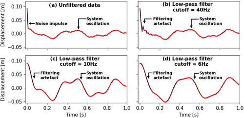
The conceptual explanation for the positive noise impulse in the RDS is that, if the acceleration response has a mean of zero, then for all positive triggering conditions there is a higher likelihood that the amplitude of the dynamic response of the system is below the trigger range rather than above the trigger range. Therefore, it is more likely that triggering of the RDT occurs due to a dynamic response with a lower amplitude than the trigger range plus a positive noise impulse. It is less likely that there is a dynamic response with an amplitude higher than the trigger range plus a negative noise impulse. This causes coherence of the noise where triggering of the level-crossing RDT occurs (the start of each data segment in the RDS) and a net positive noise impulse. If the noise is stochastic this coherence does not occur anywhere else in the segments.
When the data are filtered prior to application of the RDT, the component of the RDS associated with the free-response of the system is amplified due to the higher signal to noise ratio. However, the autocorrelation of the filtered noise impulse remains, as shown by the filtering artefacts: the additional oscillations present in Figure 2b–d. If the noise is non-white, as is common for accelerometer data,40 then, as shown by Orlowitz and Brandt,39 similar artefacts are present within the data and the autocorrelation functions or system free-response will display the autocorrelations of these artefacts as discussed in detail in Section 5. For time-domain OMA, the filtering artefact autocorrelations result in the estimation of an incorrect damping ratio as they are not a constantly damped sinusoid and cannot be accounted for in common modal analysis techniques.
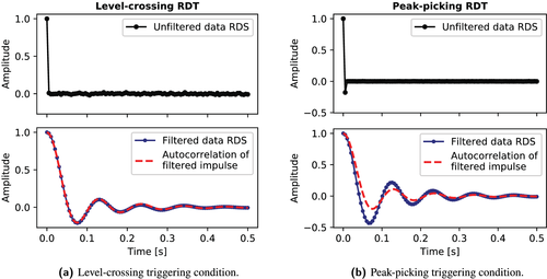
The cause of this noise impulse and its relationship to the autocorrelation of a filtered impulse can be demonstrated by analysing a data-set of white noise only with the level-crossing RDT, as shown by the top subplot of Figure 3a. The RDS of the unfiltered white noise data is the filter impulse response, with a normalised amplitude of 1 at and an amplitude close to zero at . The RDS of the filtered data is an estimate of the autocorrelation of the filtered impulse, which is equivalent to filtering the RDS of the unfiltered data with the same low-pass filter used to filter the white noise data set prior to application of RDT, as shown by the lower subplot of Figure 3a.
2.3.2 Peak-picking random decrement technique
When the peak-picking RDT is applied to a filtered white noise data set, the noise impulse remains at time , as shown in the top subplot of Figure 3b. However, a further impulse is introduced at the second time-step due to the formulation of the triggering condition. For a peak at time , the value of the amplitude at the next time-step, , must be less than the amplitude at . The inverse is true for troughs (the negative triggering condition, ). The effect of applying these conditions is that the data segments used to form the RDS are correlated at . The value of the amplitude at may be calculated by considering the probability of a given amplitude ( ) multiplied by the cumulative probability of a lower amplitude ( ) for all unique amplitudes.
The peak-picking RDS is a mixture of the autocorrelation function starting at , associated with the first peak of the filtering artefact, and the autocorrelation function at a phase lag equal to half the period of the filtering artefact oscillation, associated with all peaks of the filtering artefact not at . Therefore, the result produced by applying peak-picking RDT to filtered data is not equal to the RDT of the unfiltered data passed through an equivalent bandpass filter, as shown by the lower subplot of Figure 3b.
2.3.3 Vector random decrement technique
A common expansion of the random decrement technique as described by Asmussen and Brincker27 relies on vector-triggering; collecting samples from multiple data sets at times where the triggering condition is met within a single data set. This concept has been expanded upon here to investigate the impact of filtering on the vector RDT.
Two copies of the 2DOF example data are created, one which has been corrupted with the additive white noise, and one which has been corrupted with the same additive white noise and then filtered using a Butterworth low-pass filter with a filter order of 7 and a cutoff of 10 Hz. By using combinations of these data sets as the data for analysis and the data which defines the triggering of the RDT, distinctions can be made between false-triggering of the RDT (triggering of RDT by noise spikes) and correlations between filtering artefacts and the data itself.
Figure 4 presents the RDSs obtained for different triggering data sets (rows) and analysis data sets (columns). For comparison, all RDSs have been scaled to have an amplitude of 1 at s, with the vector RDT applied with a range-crossing trigger level of 1.5 times the standard deviation of the original data . These results demonstrate that when the triggering is based on uncorrupted and unfiltered data (original data), no filtering artefacts are induced in either corrupted or corrupted and filtered data.
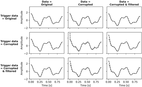
However, when the trigger data are corrupted, the noise impulse is present in the RDS of corrupted data. Filtering artefacts are present in the corrupted and filtered data, due to additional triggering of the level-crossing RDT by filtering artefacts.
Crucially, when the trigger data have been corrupted and filtered, filtering artefacts are induced in the corrupted (non-filtered) data. These filtering artefacts are induced due to the additional triggering of the RDT by the oscillations in the filtering artefacts in the trigger data and the increased likelihood of triggering by noise when the amplitude of the system response, which is correlated across the data sets, is close to the trigger level. The implications of this in practice are that where a vector RDT approach is to be utilised, or any OMA method reliant on cross-correlations, it is essential that the trigger channel is subjected to minimal filtering to prevent the dispersion of filtering artefacts to unfiltered data sets.
2.4 Covariance-driven stochastic subspace analysis
Other time-domain OMA methods are also sensitive to the filtering of the data. A widely used OMA method is covariance-driven stochastic subspace identification (SSI-COV).41 This takes the autocorrelation and cross-correlation matrices for several different data sets at varying levels of starting time lag and forms a Toeplitz Matrix before modal analysis through Singular Value Decomposition.21 The results are typically presented in stability diagrams, with increasing model order representing the number of singular values fitted. Figure 5, which compares the SSI-Cov results for the 2DOF example data before the addition of white noise (uncorrupted data), after the addition of white noise (unfiltered data) and after the addition of white noise and filtering with a variety of filter cutoffs, show that the results for filtered data are typically much worse than unfiltered data. The damping estimates for mode 1 exhibit variation in excess of 30% of the true damping value, with smaller fluctuations observed in the natural frequency estimates of both modes as the model order increases. Alongside these fluctuations and outliers, there is significant biassing of the damping estimates of the second mode of vibration for both the unfiltered and filtered data of approximately 5% across all model orders.
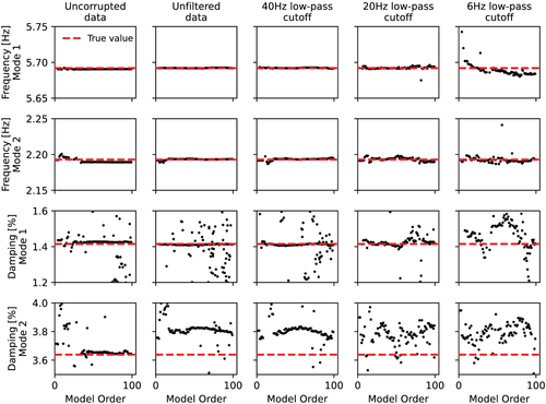
The cause of the biassing and increased variation in SSI-COV modal estimates in the unfiltered and filtered columns of Figure 5 is corruption of the autocorrelation function by the noise impulse or filtering artefacts, shown by the colour variation on the left hand side of Figure 6a which varies with the low-pass filter cutoff. These artefacts obscure the modal behaviour of the system, the low frequency colour variation in Figure 6a.
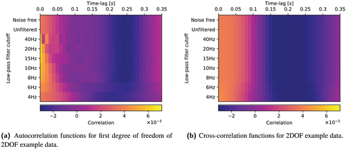
The cross-correlations, shown in Figure 6b, are unaffected by filtering of the data. As SSI-Cov makes simultaneous use of both the auto- and cross-correlations for modal analysis its results are less impacted by filtering artefacts than RDT, which typically fits each RDS independently.
2.5 Other causes of filtering artefacts
The dominant cause of filtering artefacts in time-domain OMA is almost always sensor noise, discussed at length in the previous sections, due to the low SNR of ambient vibration data. However, there are several other causes of filtering artefacts which may be encountered in OMA.
Ku et al33 demonstrated that for simulated acceleration data for a system excited with white noise and analysed with RDT, the RDS is a mixture of a systems free-response and a ‘singular point’ which is dependant on the autocorrelation matrix of the input force and the diagonal mass matrix. This ‘singular point’ is not present for displacement data33 and for real structures is usually insignificant due to the dissipation of the force through the structure.42 However, any force impulses occurring close to an accelerometer, such as is induced by heel loading on floors, will cause a measurable instantaneous acceleration response. This response will induce filtering artefacts when the data are low-pass filtered.
While the preceding sections have focused on the filtering of high frequencies using a low-pass filter, filtering artefacts are also induced by high-pass filtering of the data. When data are filtered with a high-pass filter, such as to remove long term trends within the data; or diurnal, seasonal and annual results variation, artefacts will typically occur at the start of the entire data set. This is less complex to remove as the section of the data where filtering artefacts are visible may be excluded from further analysis.
Anti-aliasing filters may introduce filtering artefacts; however, for OMA applications, these artefacts are often of insignificant amplitude due to the lower power concentrated in the high frequency range.
3 METHODS FOR REDUCING AND REMOVING FILTERING ARTEFACTS
In the previous section, the causes of filtering artefacts in ambient vibration data for two common time-domain OMA methods were demonstrated. In this section, methods of reducing filtering artefacts through the selection of appropriate filters are presented, and an alternative to filtering, the removal of the noise impulse from correlation functions, is introduced. This technique is expanded to allow removal of filtering artefacts from correlation functions. Additionally, a method of incorporating the fitting of filtering artefacts as part of the modal analysis, for use when filtering of the data is unavoidable, is presented.
3.1 Minimising the effects of filtering artefacts
All filtering of data which contains discontinuities, such as impulse responses, stochastic forcing, stochastic noise or step changes, will result in filtering artefacts. Therefore, the only way to avoid these effects is to analyse unfiltered data. However, the amplitude of the overshoot induced by filtering is related to the type of filter used. A Bessel filter results in less ringing at the expense of a less sharp filter cutoff. Similarly, a lower order Butterworth filter will result in a shorter duration of ringing but with a greater amplitude of ringing.43 More complex methodologies have been developed for minimising the effects of filtering artefacts such as the work of Gottlieb and Shu.44
Bayesian time-domain OMA methods, as described by Yuen and Katafygiotis,45 Yuen et al46 and Yang et al,47 directly avoid the introduction of filtering artefacts into the time-domain OMA as raw data are analysed without any form of pre-processing or filtering. Alongside this, Bayesian OMA methods are robust to non-stationarity in the structural response and applied forcing and may be a suitable alternative which offers greater insight into uncertainty within the modal estimates than conventional time-domain OMA methods, as discussed in detail by Yang et al.47
3.2 Trimming correlation functions
An effective alternative to filtering of the ambient vibration data is to remove or trim the component of a correlation function or an estimate of the system's free response, such as the RDS, associated with the noise impulse. The modal parameters of the system are then estimated using only the remaining component of the correlation function or estimate of the free-response after removal of the noise impulse. If the data are corrupted with white noise, the noise impulse is limited to the first data point of the correlation function or range-crossing RDS, as shown previously in Figure 2. For the peak-picking RDT triggering condition, the noise impulse is spread across the first two data points of the RDS, as discussed in Section 2.3.2.
Where the data are corrupted with non-white noise, or if the data have been filtered with a low-pass filter, the noise has a non-flat frequency spectrum. This manifests in the time-domain as either a broad impulse (a peak extending across multiple time-steps26) or as filtering artefacts extending across multiple time-steps. These may also be trimmed by first identifying the section of the correlation function or RDS corrupted by the noise peak or filter artefacts, either visually or through knowledge of the likely duration of the artefact ringing, and then limiting the modal analysis to where the amplitude of the noise peak or filter artefacts have decreased to a negligible amplitude, as shown in Figure 7. The modal parameters of the system may then be estimated through analysis of the remaining section of the free-response estimate or correlation function, the non-shaded section within Figure 7, without biassing of the modal parameters induced by the noise impulse.

An amplitude threshold of 5% of the initial amplitude of the filtering artefact is recommended to reduce the biassing which the filtering artefacts introduce. However, the selection of an appropriate length of the correlation function or RDS to be trimmed is dependant on a wide range of factors. If a mode contains large numbers of modes with low amplitudes, a lower amplitude threshold of 1% is advised to ensure that the ratio between the amplitude of each modal component and the amplitude of filtering artefacts is reduced as far as is reasonably practicable. This approach is not suitable if a system contains heavily damped modes, as the longer trimming length required to meet the amplitude threshold for reduction of the filtering artefact may negatively impact the modal identification. In such situations, it is advisable to alter the filter parameters so as to minimise the ringing which occurs as a result of the filtering, or use the indicative noise profile approach presented in the next section.
3.3 Removal of filtering artefacts through use of an indicative noise profile
Where filtering of the data for OMA is required, filtering artefacts are unavoidable. Alongside the selection of a filter to minimise ringing, a novel approach is proposed in this section whereby the autocorrelation of a filtered impulse is fitted as part of the modal analysis. If the amplitude and shape of the noise impulse is known, a filtered noise impulse can be numerically generated based on the expected filter response and subtracted from the autocorrelation functions, or RDS free-responses, prior to the modal analysis. However, a key limitation of this approach is that the exact parameters of the filtered noise impulse may not be known prior to analysis.
A similar approach can be employed to remove the effects of bandpass limited stochastic forcing by estimating the frequency spectrum of the forcing, using the inverse Fourier transform to generate an equivalent time-domain forcing function and fitting this to the autocorrelations or RDSs. The scaling of INP can be improved upon during the modal analysis by scaling based on multiple points, through repeated iteration of the process of estimating and modal analysis of the correlation function or through directly estimating the scale factor as part of the modal analysis. However, for systems dominated by a single mode of vibration, the simple one-step scaling presented here produces satisfactory results.
4 SIMULATED DATA TESTING
4.1 Data generation
To quantify and separate the uncertainty inherent in analysing systems under ambient excitation due to the unknown forcing of the system47 from systematic biassing of the modal estimates introduced due to filtering of the data, 10,000 numerical data sets were independently generated using the Newmark Beta method32 for each DOF of the 2DOF system the mass and stiffness matrices for which were presented in Section 2.2. For each 60 min data set, sampled at 100 Hz ( samples per DOF), the values of and were randomly selected from a uniform distribution between 0.1 and 20,000 N/m with the constraint that both natural frequencies of the system must fall between 0.5 and 25Hz. The values of were randomly generated from a uniform distribution between 0 and 10. The values of were randomly generated from a uniform distribution between 0 and 0.1. An additional condition was imposed which ensured the values of and selected resulted in damping values for both modes less than 10% of the critical damping. Through the methodology described above, 10,000 independent data sets were generated each with a unique set of frequency and damping estimates, histograms of which are shown in Figure 8.

Additive white noise was independently added to the displacement data from both DOFs to achieve a modal signal-to-noise ratio (SNR)1 randomly selected with equal probability between 0.5 and 100. A wide SNR range was selected so as to assess the impact of filtering on modal parameter estimates when the level of noise within the data is low, and it might be expected that the any biassing due to the filtering artefacts would be minimal.
A 2DOF system was selected for the simulated data testing to allow the variation in modal parameters due to filtering artefacts to be isolated from other sources of uncertainty within time-domain operational modal analysis. These sources of uncertainty for higher order systems include the selection of an appropriate model order during the modal analysis, and the selection of a random decrement signature length which balances the competing interests of modal identifiability with the higher ratio of noise to system response which is typical for longer random decrement signatures or correlation functions.27 While filtering artefacts can be isolated for higher order systems, parsing the impact which these filtering artefacts have on the uncertainty and biassing for the modal estimates of individual modes from the other sources of uncertainty and biassing within the analysis is complex and beyond the scope of this current study.
4.2 Data analysis
Copies of each data set were filtered using a butterworth low-pass filter (order = 7) with a range of cutoff frequencies. Each filtered data set, alongside the unfiltered data sets, were analysed with the vector RDT with a range-crossing triggering condition27 of 1 to 2 standard deviations of the trigger data. Each RDS was analysed with the Matrix Pencil method,48 with the model order increased until the coefficient of determination ( 34) between the RDS and the fitted signal was greater than 0.99. Separately, the unfiltered and trimmed RDS (the unfiltered RDS with the data point at time excluded) was also analysed.
4.3 Simulated data—Mode detection efficacy
Filtering artefacts may significantly impact the ability of time-domain operational modal analysis to detect all modes of vibration within correlation functions and random decrement signatures, as shown in Figure 9. Presented in this figure is the number of modal estimates where (i) the true natural frequency of the mode is below the low-pass filter cutoff, (ii) the error in the frequency estimate is below 7.5 Hz and (iii) the error in the damping estimate is less than 2% of the critical damping. The values for the allowable frequency and damping error are based on the 95% confidence interval for the distributions of modal estimates presented in Figure 8. As expected, the number of first and second order modes detected decreases as the low-pass filter frequency is decreased due to modal components being filtered out. However, there is a significant drop in the number of second order modes detected when the low-pass filter frequency is between 10 Hz and 20Hz. This is driven by the filtering artefacts dominating the RDSs generated with data from the second DOF. Therefore, the second largest component fitted to the RDS corresponds to components fitted to the filtering artefact, not the second mode of vibration.

4.4 Simulated data—Frequency estimates
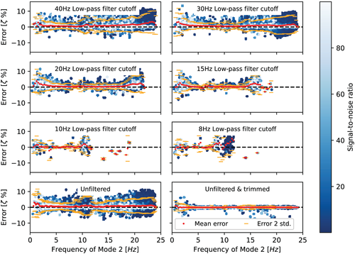
The error in the frequency estimates of the simulated data for the first mode (the fitted modal component with the largest amplitude) and the second mode (the fitted modal component with the second largest amplitude) are plotted in Figures 10 and 11. In each figure, the results are presented for a range of low-pass filter cutoffs, the unfiltered condition, and the unfiltered condition where the first point of the RDS is trimmed prior to the matrix pencil fitting. For each fitted mode, the error is based on the closest natural frequency of the system. Results where the true natural frequency of the mode is above the low-pass filter cutoff are excluded from these plots. The colour of the data point corresponds to the SNR of the data prior to filtering, with darker colours corresponding to a lower SNR. A moving average of the frequency estimates across all SNRs, based on a window width of 1.5Hz, is shown with red markers, with 2 standard deviations of the windowed results shown as orange markers.
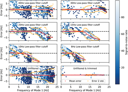
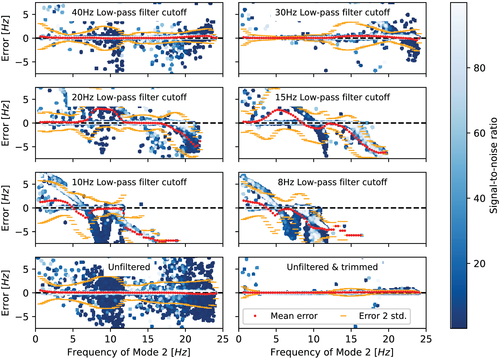
It is clear that the unfiltered and trimmed RDS is the most consistently accurate approach, with the mean absolute frequency error of the unfiltered data in the plotted range (0.084 Hz) being 235% higher than for the unfiltered and trimmed data (0.025Hz) for the largest fitted component, and 198% higher for the second largest fitted component (0.36 Hz vs. 0.12 Hz). The error is consistently higher for the second largest fitted component, which usually corresponds to the second mode of vibration. This is likely due to the lower amplitude of movement for the second mode of vibration. This leads to a higher ratio of the filtering artefact amplitude (which is primarily dependant on the noise level of the signal) and the modal amplitude, which causes larger errors in the frequency of the fitted signal component. For the same reason, the data sets with lower SNR have higher errors across all filtered and unfiltered (non-trimmed) results; a lower SNR leads to a higher ratio of the filtering artefact amplitude to the amplitude of the modal component within the RDS. However, as the noise impulse from a white noise process is only present in the first data point of the RDS and is therefore excluded from the unfiltered and trimmed RDS analysis, there is a much weaker correlation between the SNR and the error in the frequency estimates.
As might be expected, the largest errors in the frequency estimates occur at the higher frequencies and when the natural frequency of the system is close to the low-pass frequency cutoff. The filtering artefacts cause the distinctive linear variation in error as the natural frequency approaches the cutoff frequency. However, there is no clear biassing in the frequency estimates if the cutoff frequency is more than a few Hz from the natural frequency of interest.
4.5 Simulated data—Damping estimates
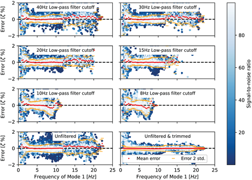
The error in the damping estimates, provided as the percentage of critical damping , is presented in Figures 12 and 13. For each fitted mode, the error is based on the closest natural frequency of the system, with results where the true natural frequency of the mode is above the low-pass filter cutoff excluded from the analyses.
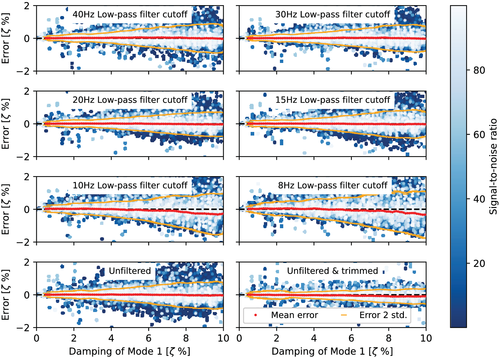
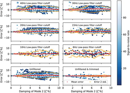
As with the frequency estimates, the unfiltered and trimmed results lead to damping estimates which have a mean absolute error in the plotted ranges which is 56% lower than the unfiltered results (0.11% error vs. 0.18% error) for the largest component of the fitted RDS and 774% lower for the second largest fitted component (0.14% error vs. 1.22% error). The error in the unfiltered and trimmed damping estimates is not correlated with the SNR, while the unfiltered and low-pass filtered results show increased variance in the damping error with decreasing SNR. In practice, this increased variance with decreased SNR may easily be mistaken for amplitude-dependant damping behaviour, as high amplitude signals will have a higher SNR and may be expected to have a lower damping error.
Significant biassing is present in the low-pass filtered and unfiltered results for the second largest component of the fitted RDS, as shown by the non-zero mean error in the damping estimate plotted in Figure 13. These results show a consistent overestimation in the damping of the system which increases as the true system damping increases. Significantly, as shown in Figures 14 and 15, the error in the damping estimate induced by the filtering artefact is independent of how far the natural frequency of the mode is from the low-pass filter cutoff for both modes of vibration. The implication of this in practice is that damping estimates may be negatively impacted by filtering even when the mode of vibration is far from the filter cutoff frequency. For example, it can be seen that there is significant biassing and errors in the damping estimates for modes of vibration at 10 Hz, even when the low-pass filter cutoff is at 25 Hz, with these errors being of a similar magnitude to that of the unfiltered data and having a variance which is twice as large as the errors of the damping estimates from the unfiltered and trimmed RDS.
5 REAL-WORLD DATA APPLICATION
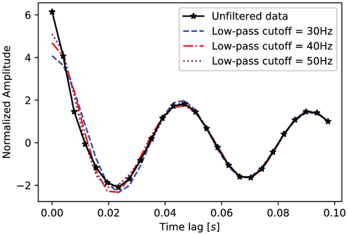
To verify that filtering artefacts impact all data, and not just simulated data, 100 min of vertical acceleration data, sampled at 256 Hz, was collected from the underside of a two-way spanning concrete slab subject to footfall excitation. While this structure is dynamically simple, it is indicative of a typical application of OMA for the analysis of floor vibrations at the serviceability limit state49 and allows the impact of filtering artefacts on the modal estiamtes to be robustly and accurately isolated. The range-crossing RDT, with a trigger range of 0 to , was used for the analysis after the application of a Butterworth filter of order 7 with various level of low-pass filter cutoffs. From Figure 16, it can be seen that there is a slight corruption introduced into the RDSs for the filtered data. To allow comparison of the RDSs, all RDSs have been normalised to give an amplitude of unity at s.
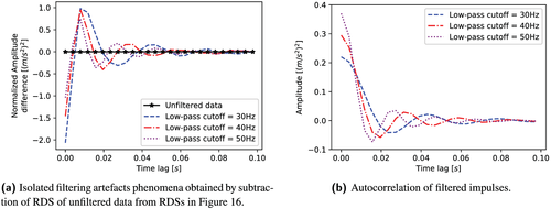
By subtracting the normalised RDS of the unfiltered data from that of the filtered data, shown in Figure 17a, it can be seen that the cause of this corruption is the autocorrelation of the filtering artefacts. A close approximation of these filtering artefacts can be recreated as shown in Figure 17b through filtering an impulse function using the same sampling and filtering parameters.
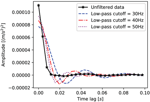
However, there are key differences between the isolated filtering artefacts and the filtered impulses caused primarily by the non-white nature of the sensor noise. This non-white noise can be identified by applying the RDT to an INP, a section of data collected when the slab is not excited. The RDSs for the filtered and unfiltered INP are shown in Figure 18. The presence of a noise impulse lasting several samples indicates that the noise has a non-uniform power spectrum and contains significant low-frequency components. This is a common feature of the noise profiles of both piezoelectric and MEMS accelerometers.40
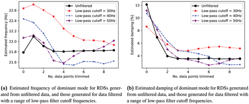
The impact of the extended noise impulse is that the fitted parameters of the system changes depending on which part of the RDS is fitted, as shown in Figure 19a,b. As the majority of the noise impulse is excluded after the trimming of the first three data points from the unfiltered RDS, the fitted modal parameters stabilise at a constant value. However, as the filtering artefacts have significant amplitude past three data points, the modal parameters do not converge to a constant result.
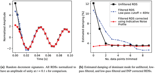
The removal of the filtering artefacts from the two-way spanning slab data using an INP is demonstrated in Figure 20a. Five minutes of data where there was no excitation of the slab were isolated, filtered and analysed through the range-crossing RDT with limits of 0 and to create the filtered INP RDS, , which was scaled using Equation 8. By scaling and subtracting the filtered INP RDS from the RDS of the filtered data collected when the slab was excited ( ), the majority of the filtering artefacts are removed, as seen in Figure 20a, and the biassing of modal estimates greatly reduced, as shown in Figure 20b. This allows analysis of the slabs dynamic response with minimal corruption of the modal estimates by filtering artefacts.
6 CONCLUSION
Due primarily to the presence of noise within the autocorrelation function, or estimates of a systems free-response, filtering of data for use in time-domain operational modal analysis induces filtering artefacts. Within this paper, we have demonstrated how this results in higher errors in damping estimates for systems with higher damping ratios, or data which have a lower signal-to-noise ratio, and that these errors may be on the order of hundreds of per cent of the true damping value. Using acceleration data collected from a two-way spanning concrete slab subject to footfall excitation, the filtering artefacts have been isolated. A range of techniques for minimising the effects of filtering artefacts in time-domain operational modal analysis have been discussed, and two novel practical solutions, in the form of either excluding sections of the autocorrelation functions corrupted by noise impulses/filtering artefacts from the modal analysis or by generating estimates of the filtering artefacts using indicative noise profiles, have been presented and their application demonstrated using numerical and real-world data.
ACKNOWLEDGEMENTS
The authors would like to thank Professor Iain Murray at the School of Informatics, University of Edinburgh, for his early input into the development of this paper. Support for Z. Wynne was provided by an EPSRC Doctoral Training Partnership Studentship (EP/R513209/1). Thomas P. S. Reynolds is supported by a Turing Fellowship. For the purpose of open access, the author has applied a Creative Commons Attribution (CC BY) licence to any Author Accepted Manuscript version arising from this submission.
AUTHOR CONTRIBUTIONS
Zachariah Wynne: conceptualization (lead); formal Analysis (lead); investigation (lead); visualization (lead); writing – original draft (lead); writing – review and editing (equal); James R. Hopgood: conceptualization (equal); writing – review and editing (equal); Tim Stratford: supervision (equal); and Thomas P. S. Reynolds: conceptualization (equal); supervision (equal); writing – review and editing (equal).
Open Research
DATA AVAILABILITY STATEMENT
The data that support the findings of this study are available from the corresponding author upon reasonable request.


