Funding: This work was supported by the Austrian Science Fund (grant DOI: 10.55776/I5799); the European Commission (no. CZ.02.01.01/00/23_025/008686); and the Czech Science Foundation (grant 22-15684L).

About

Sections

PDF

Tools

Share a link

Email
Wechat
Bluesky

ABSTRACT

Correspondence analysis (CA), a well-known method for analyzing the relationships between rows and columns of a table, has been reformulated to link to the logratio methodology of compositional data by using the limiting case of the power transformation. The resulting methodology investigates relative rather than absolute information, and it is invariant with respect to rescaling rows or columns. The latter properties also hold for the analysis of compositional tables, where the table is first decomposed into an independent and an interaction part. It is shown that the analysis of the interaction part is equivalent to CA, but in addition, the variance contributions can be determined. Both concepts also allow for an inclusion of weights to suppress undesirable variance, and it is shown that the equivalence between weighted CA and the analysis of weighted compositional tables again holds. This equivalence allows us to make use of the mathematical framework of weighted compositional tables, the so-called Bayes spaces, to get a deeper understanding of CA and to construct extensions to multi-factorial tables (cubes, etc.).

1 Introduction

Correspondence analysis (CA) is a prominent method in exploratory data analysis, with the aim to analyze the relationships in a contingency table with either discrete-valued or continuous entries [1-3]. The main idea is to subtract the product of row and column marginals from the proportional representation of the contingency table (referring to the “correspondence matrix”), rescale it to the totals of the marginals, and proceed with a singular value decomposition (SVD). This yields row and column information of the table, which can be visualized in order to study their relationships.

An interesting case is studied in Greenacre [4], where in a first step the elements of a

contingency table

are transformed with the Box–Cox transformation [5] with power parameter

()

approaches zero, CA is essentially (in the limiting case) based on log-transformed data, and this provides the link to a compositional data analysis of the table [4]. Generally speaking, compositional data are understood as observations carrying relative information [6], and also CA makes use of a decomposition of a specific kind of relative information. If log-transformed data are used, an SVD of row- and column-wise centered data allows to construct the so-called compositional biplot [7], with the goal to visually study the relationships between rows and columns of the table.

In the context of compositional data, row centering is presented by the so-called centered logratio (clr) coefficients [6], defined for the ith composition

, that is, the ith row of a table

with entries

(

and

), as

()

With the clr coefficients, the compositional data are moved isometrically from their original sample space, endowed with the Aitchison geometry, to the real space (see, e.g., Pawlowsky-Glahn et al. [8]), where indeed standard SVD after (column-)centering results in a meaningful representation of loadings and scores in a biplot. Since logarithms of ratios are involved, this kind of procedure is generally known under the name logratio approach (see, e.g., Pawlowsky-Glahn et al. [8], Greenacre [9], and Filzmoser et al. [10]).

Recent developments in compositional data analysis, however, enable to proceed further with this limiting case. In particular, the concept of compositional tables opens up new possibilities also for the analysis of relative information in contingency tables [11-13]. As an example, a simple compositional table could be the number of employed people in a region, where the rows are determined by part-time and full-time employment, and the columns by males and females. If one is interested in comparing and analyzing different regions, relative rather than absolute information needs to be considered, as the absolute numbers would essentially be determined by the population size.

To make the link to the mentioned limiting case of correspondence analysis as presented in Greenacre [4, 14], in this paper only one table is considered, and the interest is again in identifying relationships between rows and columns. More specifically, the possibility of a decomposition into two tables, an independent and an interaction part, will be utilized. The former assumes independence of the row and column factors and consists of a product of the respective marginals, and the latter contains the information about their interaction and is numerically equal to the matrix used in correspondence analysis. However, the construction of the interaction table enables to completely filter out in a geometrically meaningful way the independent part from the original table, and thus provides direct pathways to analyzing the remaining interactions. Besides the description of CA from the perspective of compositional tables, the paper also introduces a new mathematical framework for weighting parts of a compositional table and, consequently, for weighted CA, and establishes a solid foundation for an extension to the multi-factorial problem.

The structure of the paper is as follows. In the next section, a key relationship between double-centered log-transformed data and the interaction part of a compositional table (correspondence table) is derived. In Section 3, we generalize the findings to weighted versions of the methods and investigate their equivalence. Section 4 shows that the important property of distributional equivalence also holds for the logratio approach. Numerical experiments which reveal the advantages of using weights are presented in Section 5, and the final Section 6 concludes and provides an outlook to further extensions.

2 Unweighted CA

This section recalls classical (unweighted) CA as well as logratio analysis (LRA), performing CA on log-transformed data. Moreover, we present the concept of compositional tables and show the link to LRA.

2.1 Logratio Analysis (LRA)

Let the

contingency table

be given, either in form of counts or as continuous numbers, and let

, be the respective matrix of proportions. Classical CA is typically based on an SVD of the residual matrix

()

where

and

are vectors of row and column marginals of

, with

a vector of

values of 1, and

and

If the rows of the matrix

represent realizations of a

-part compositional vector, that is, a vector with positive values carrying relative information [6], the unweighted LRA is given by an SVD of the double-centered matrix

[15]. Row-wise centering of

can be understood as the clr transformation of the rows of

[8], where the entries of

, are given as

After additional column centering we obtain the matrix

with entries

()

which is subsequently decomposed with SVD. The matrix

has mathematically the same entries as the clr representation of the so-called interaction table, which is introduced in the following section.

2.2 Compositional Tables

The two-factorial extension of the concept of compositional data to compositional tables [11, 12] treats as one data object, which follows the idea of CA. A convenient property of the approach is that the table can be orthogonally decomposed into an independent and an interactive part with respect to the Aitchison geometry [11]. This can be written as , with standing for the entry-wise product, known in the compositional context as the operation of perturbation.

The independent table

follows the situation of independence between row and column factors, and its entries are given as the product of the geometric marginals,

Thus, the geometric marginals replace the arithmetic marginals and used in classical CA, see Equation (3). The geometric marginals have an important property: they are orthogonal projections of the compositional table on the information contained in its rows and columns, see Genest et al. [16] for more details. Note that in case of truly independent row and column factors, both the arithmetic and geometric marginals are equivalent [11], which underpins the reasonability of their definition.

The remainder of

is contained in the interaction table

with entries

This table carries information on associations between row and column factors. Therefore, it can serve as a natural compositional alternative to matrices used in classical CA (matrix of standardized residuals or matrix of Pearson contingency ratios).

The clr representation of a compositional table

, has components

()

and the orthogonal decomposition still applies, as

can be decomposed into

. The matrices

and

are the clr representations of

and

, with entries given as

The clr representation turns the geometric marginals of

into the (scaled) arithmetic margins of

, which can be written as

()

and

()

The entries of

are thus equal to

()

Equations (4) and (8) reveal that

()

and thus LRA is equivalent to an SVD of the clr-transformed interaction table. However, the equivalence is achieved just numerically, but from a mathematical perspective the models are not the same. While the former approach understands

as a realization of

observations, the latter treats the entire matrix

as one observation.

For both the independent and the interaction table, the clr coefficients can also be derived directly from the elements of the original input table

()

de Sousa et al. [17], where stands for the geometric mean of the entire compositional table. Moreover, has uniform (zero) marginals and is thus margin free as mentioned in Greenacre [4] (Result 1).

Due to the orthogonality of the independent and interaction tables, Pythagoras' decomposition of squared norms holds [16]. Specifically,

()

where

is the usual Frobenius norm of a matrix. Accordingly, by computing

()

also known under the term “simplicial deviance” [11], one can easily (and in a mathematically justified way) decipher the amount of information stored in the interaction table.

2.3 CA of a Compositional Table

The equivalence of the double-centered matrix

and the clr-transformed interaction table

, see Equation (9), implies that CA is obtained by an SVD of the interaction table,

()

with orthogonal matrices

and

, and the (rectangular) diagonal matrix

with

. Double centering of

guarantees that the columns

, and the columns

, have zero totals, so they can be perceived as clr transformations of the respective row and column compositions. The SVD can then be written as

which results in a univariate decomposition of the interaction table (which could possibly be back-transformed to the original space). Clearly,

and therefore

can be considered as proportion of information (variance) explained by the kth factor—of course, within the interaction part. By considering Equation (11), one can however relate the factors also to the overall table through

. Finally, plotting the first two columns of

and

, possibly rescaled by

and

, together in a planar graph then informs about interactions between row and column factors, as in classical CA.

3 Generalization: Weighted CA

In real-world applications, the information on the actual data structure can be blurred due to problems related to sampling of the initial data matrix. The structure can be affected by measurement errors, unbalanced sizes of samples defining the rows, or the presence of cells with low observed value; see, for example, the example in Greenacre and Lewi [15, sec. 2]. Also, in recent work, weighting of rows and columns in CA is proposed and considered useful [18]. In the logratio context, weighting can be used to give less importance in the analysis to components with small proportions that often have high variance on the logratio scale [4, 15, 19]. In the following, we will compare weighted CA/LRA with a weighted CA version for compositional tables.

3.1 Weighted CA and LRA

Weighting in CA is commonly carried out by introducing row and column weights (typically row and column arithmetic marginals) in the double-centering stage. The vectors and forming the correspondence matrix , see Equation (3), are computed with respect to given weights. Consequently, weighting propagates also into the approximation stage, so that fitting is done by weighted least squares [15]. According to Greenacre and Lewi [15], weighted CA can alternatively be motivated by a matrix of Pearson contingency ratios , with , , . With the weights in form of the row and column marginal vectors and , and the matrices and , see also Equation (3), one can carry out an SVD of to perform a weighted CA, which then is equivalent to the weighted form of LRA. There are also other important contributions on the equivalence between correspondence analysis and weighted LRA indices: Greenacre [4] provided an empirical description of the respective transformation, Choulakian [20] later presented a mathematical formulation and proof, referring to it as Greenacre's Theorem, and Greenacre [14] subsequently offered an alternative mathematical formulation with a similar proof.

The weighted LRA starts with double centering of

by weighted means. When

and

are vectors of normalized row and column weights (

), weighted LRA is based on an SVD of the matrix

()

with

and

being diagonal matrices of weights. The result remains unchanged if a constant is added to the rows or columns of

, as it vanishes through the double centering. The matrix

is therefore equivalent to the matrix of log-transformed Pearson ratios

. Moreover, since a logarithm of

can be approximated by

via Taylor approximation, the matrix

is similar to

if all

. Finally, the shift by

again vanishes through the double-centering and the weighted LRA and CA approaches are therefore equivalent if the observed and expected values (nearly) coincide, that is, if the analyzed structure is rather independent. The detailed derivation is given in Greenacre and Lewi [15]. Additionally, the weighted LRA is also equivalent to spectral mapping, described, for example, in Lewi [21], and to the weighted version of CA of a compositional table as detailed below.

3.2 Weighted CA of a Compositional Table

Let be an matrix of positive weights satisfying , that is, of a structure which is in agreement with weighted LRA [15] and which also corresponds to the product reference measure as used in Genest et al. [16]. Among other options, the vectors of weights and can be given by the arithmetic or geometric marginals, and possibly rescaled to unit sum. However, the rescaling would affect merely the scale of the final result, not the (weighted) data structure itself.

The mathematical framework for the weighted analysis of compositional tables, and consequently for the weighted CA of a compositional table, is provided by Bayes spaces [22, 23]. The fundamentals of the weighted analysis of vector compositional data are given in Hron et al. [19] and can be directly generalized to the two-factorial case, as described here. Weighting in the Bayes space framework is in general understood as a shift, in compositional terms a perturbation-subtraction (denoted as

) of the object with weights. More specifically, for a compositional table

and a matrix of weights

, the weighted compositional table

has elements

()

and it is represented in a weighted Aitchison geometry which honors scale invariance of the table and its weights. The scale of the weights only propagates in metric concepts, like in the weighted Aitchison distance between two tables

and

()

depending on rescaling of

, the sample space of the tables either shrinks (

) or expands (

). Note that the weighted Aitchison distance (16) corresponds to quite an extent to the heuristic approach to weighting the distance in compositional data analysis, cf. Greenacre and Lewi [15, sec. 2]. The main difference is the initial shift of the correspondence table by the compositional table of weights, which can be understood as shifting the data to a new representation where the matrix of weights plays the role of the new origin. Accordingly, the weighted observations now indicate how much they differ from the a priori information represented by the weights. This gives an additional theoretical frame to the setting from Greenacre and Lewi [15] which enables to generalize, for example, the Pythagoras' decomposition or the distributional equivalence from the unweighted case [16, 24]. Despite differences in the weighting pipeline, the final effect is of course the same: cells having higher weights yield more emphasis in the analysis, compare with Talská et al. [24] and fig. 2 therein.

The weights propagate into clr coefficients of the whole table as well as its independent and interaction parts. The entries are given by

()

where the weighted geometric mean of

is defined as

and likewise for row and column geometric means. Note that such definition of marginals corresponds, up to normalizing with the sum of weights, to weighted arithmetic marginals in the log-scale as defined in Greenacre and Lewi [15, sec. 2, Step 1] or Choulakian et al. [25]. The rescaling by

guarantees that the resulting weighted clr coefficients are represented in the (unweighted) Euclidean geometry, and are thus ready for further processing using ordinary tools of multivariate statistics [19]; compare also with Greenacre and Lewi [15, sec. 2, Step 2]. The entries of the interaction table are (up to rescaling by

)

()

and they play an essential role in CA. Moreover, if we denote sums of the weights

and

, respectively, and their normalized versions as

and

, the clr representation of the weighted interaction table turns to

()

Therefore, the weighted version of CA based on a log-transformation (LRA) and the decomposition of a compositional table are equivalent.

It follows directly from the general case [16] that the weighted independent and interaction parts are again orthogonal, and therefore Pythagoras' decomposition

()

holds, similar as in Equation (11). Here, a key component is the use of the product reference measure, which is essential also for derivations performed in Genest et al. [16]. Consequently, Equation (21) can be used for diagnostics related to an ordinary SVD of

, analogously as in Section 2.

3.3 Choice of Weights and Implications

The most appealing case of weighting is definitely the one with the standard arithmetic marginals of the original contingency table or its proportional representation, the correspondence matrix, as and . Due to scale invariance of weighting in compositional tables, both representations are now equivalent and the rescaling results just in a shrinkage or an expansion of the weighted space [19]. There are good reasons for weighting in the logratio CA: due to the logarithmic scale, row or column factor instances (variables) with small presence engender large variability, which is often a rather undesired effect [15]. The weighting also combines advances of both approaches: simple interpretability of arithmetic marginals as weights is complemented by geometric marginals (i.e., arithmetic margins in the logarithmic scale) which are necessary to develop both important theoretical and practical consequences of the decomposition into independent and interactive parts.

4 Distributional Equivalence of the Logratio Approach

Distributional equivalence is a natural requirement for CA and, more generally, for analyzing any ratio-scale data, including compositional data and compositional tables. In the former case, this requirement was already emphasized in the seminal work on CA [1], and it was further elaborated by Greenacre and Lewi [15], who used the formulation: If two columns (resp., two rows) have the same relative values, then merging them does not affect the distances between rows (resp., columns). An important aspect is what we understand under merging in the context of ratio-scale data. As the logarithm naturally moves the data from the ratio-scale to the interval-scale [26], the simple aggregation should be done there, possibly rescaled by the number of components. In the original scale this is just the geometric mean, which is promoted in the literature also for a geometric reasoning [27]. Likewise, in CA, the distributional equivalence is related to an amalgamation of rows/columns in case of their proportionality, which should be done again for similar reasons in the log-scale. Due to scale invariance of compositional tables, from the perspective of the original scale, it is equivalent if the aggregation is done in the log-scale or in the clr space. Then, if any two rows (or columns) of a compositional table carry the same relative information, or in other words, if they are a constant multiple of each other, it is expected that the logratio CA keeps unchanged irrespectively whether these rows (columns) are aggregated.

In case of compositional data, replacing two compositional parts with their respective geometric mean essentially means that the information contained in the ratio between these two parts is removed, and even more, it can be considered as the orthogonal projection of the original composition to the subspace of the remaining information [28]. Consequently, when considering a sample of compositional data, distances among the original compositions and among their aggregated counterparts remain the same. It is only important to keep the original dimensionality of the data; otherwise, the subcompositional dominance [8] necessarily applies.

The thoughts of Greenacre and Lewi [15] on distributional equivalence can also be reinterpreted to the case of compositional tables. In particular, in case of proportional rows (columns), the interaction part should remain unchanged irrespectively whether these rows (columns) are aggregated or not. This can be easily demonstrated. Without loss of generality., let the first two rows of the compositional table

be proportional, which means that

for any

and

. If each of these rows is replaced by

, from the scale invariance property it directly follows that the column marginals are the same as in the non-aggregated version of the table. For row marginals we need to consider that

The row geometric marginals for a table, where the corresponding elements of the first two rows are replaced by their geometric means, can then be expressed as perturbation of the original column geometric marginal by the -part composition . From the Yule perturbation property (cf. Genest et al. [16, Proposition 7]) it then follows that the interaction table remains unchanged.

Similarly, the same arguments can also be made for the weighted case, with

. By the aggregation of rows we now understand their replacement by the weighted geometric mean, and from the equality

it follows that the weighted column marginals are the same irrespective of the row aggregation. For row marginals, we need to consider that

and that the geometric mean of an aggregated row equals

. The aggregated row marginals can therefore be obtained by the perturbation of the non-aggregated ones by

, which again results in an equivalence of the respective interaction tables. Finally, the proportionality of the rows can be still traced back to the original (unweighted) table, since

5 Numerical Experiments

In this section we aim to complement previous work by Greenacre and Lewi [15] and compare the stability of the results for the unweighted and weighted version of LRA. Accordingly, we perform an SVD of the matrices and . For the weights we will use the arithmetic marginals of the original table.

5.1 Bootstrapping Tables

The main idea is to draw bootstrap samples from the original table , where we assume that are integer-valued. Each entry and is replicated times, forming the rows of a data matrix in “long format,” with rows. Then we draw a bootstrap sample, that is, observations with replacement, and the resulting long format representation is aggregated to a table format, with the same rows and columns as the original table. Call this bootstrapped table , for , where the number of bootstrap tables can be large (e.g., 1000). The unweighted version for the original table results in a decomposition of the interaction table with the singular vectors arranged in and , respectively, see Equation (13), and similarly, we obtain the matrices and for the interaction table of the bootstrapped table. For the weighted version we obtain the interaction table , see Equation (20), and the orthonormal matrices and with the left and right singular vectors, respectively. Equivalently, we obtain for each bootstrapped weighted interaction table the corresponding matrices with the singular vectors and .

5.2 Comparison by the Principal Angle

The results are compared by the principal angle between subspaces, as introduced in Björck and Golub [29] and implemented as the function angle() in the R package rospca [30]. Denote by

and

two orthonormal bases, where the number of basis vectors in

is less or equal the number of basis vectors in

. Then, the principal angle

between the corresponding subspaces is computed as

()

where

corresponds to the largest singular value of the projected matrix [29]. Here, the angle was already scaled to the interval

, where 0 means that the smaller subspace is embedded in the bigger one (or they span the same space).

In the following experiments, we compare the angle of the results for the original (weighted) table with those for the bootstrapped (weighted) tables, where we use all singular vectors in the first case, but only the first two singular vectors in the second case. Thus, the idea is to see whether the results usually shown in a 2D plot for the bootstrapped version are related or even embedded in the space spanned by the results of the original data version. Note that the angle will be 0 when comparing the singular vectors of the smaller dimension of , and thus we will report , and similarly for the weighted versions.

5.3 Spanish Health Survey Data

This data set originates from a Spanish health survey and it was analyzed in Greenacre [31]. Table 1 presents the data that have been used for CA. The rows refer to different age groups, and the columns refer to the health status as perceived by the 6371 respondents, with the corresponding frequencies in the cells. In contrast to the analysis presented in Greenacre [31] based on the frequencies, we are here interested in relative information, and thus treat the table as a compositional table. Some categories contain small frequencies, which can introduce a lot of undesirable variability in an unweighted analysis.

TABLE 1. Data derived from the Spanish national health survey.

Age group	Very good	Good	Regular	Bad	Very bad
16–24	243	789	167	18	6
25–34	220	809	164	35	6
35–44	147	658	181	41	8
45–54	90	469	236	50	16
55–64	53	414	306	106	30
65–74	44	267	284	98	20
75+	20	136	157	66	17

Figure 1 presents the results from unweighted and weighted LRA. There are several changes visible, such as an exchange of the positions of “Very bad” and “Regular,” but also of “55–64” and “65–74.” The bootstrapped tables will introduce even more uncertainty in the categories with small frequencies, and the stability of the results will be investigated in the following. It is also interesting to compare the explained variances, shown along the axis legends in the plots of Figure 1: The first numbers refer to the explained variance within the interaction parts, while the second numbers refer to the proportion of explained variance from the overall (weighted) clr table. In the latter case, weighting here leads to a much higher variance proportion because the weights shift the information to a new origin which removes a lot of the information from the independent part.

Details are in the caption following the image — **FIGURE 1**
Open in figure viewer PowerPoint

Spanish health data: Results from unweighted (left) and weighted (right) LRA.

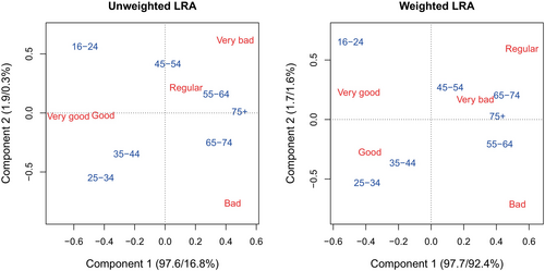
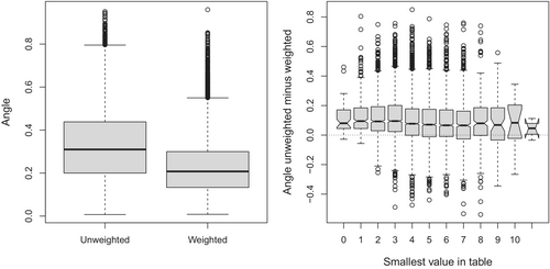
Figure 2 presents the results from the bootstrap experiments, as described above. It can happen that zero frequencies occur in a bootstrap table. Such values were replaced simply by 2/3 to add minimum possible variance [32]. The boxplots in the left plot compare the angles of the unweighted LRA with the weighted version, and it can be seen that the angles are clearly smaller for the weighted LRA. The right plot shows for each bootstrap replication the difference of the angle between the unweighted and the angle of the weighted version as boxplots, together with notches for confidence intervals around the median. The boxplots are split up into bootstrap experiments where the smallest value in the bootstrapped table was 0, 1, 2, and so forth, which is shown on the horizontal axis. This reveals that the medians of the differences are positive, and that they tend to be higher if the smallest value is smaller. Thus, weighting stabilizes the results, particularly if there are small frequencies involved.

5.4 Further Data Sets

We investigate for several other data sets known from the CA literature the stability of the results based on the bootstrap procedure as described above. For the choice of the data sets, we considered different aspects, such as the dimension of the table, values close to zero, low counts in some rows or columns, and so forth. Of course, here we consider the table information as compositional. As before, we will present the results from the bootstrap procedure in terms of the difference between the angle of the unweighted and the weighted version, see Figure 3.

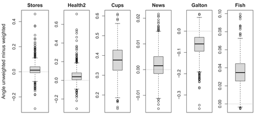
Stores: Age distribution in food stores, used in Chapter 15 of Greenacre [3]. This small data set with counts consists of 5 stores (rows) and 5 age groups (columns). The counts are relatively balanced among the cells, with the smallest value of 8 and the largest of 69. The weighted version shows a slight improvement in stability of the results when compared to the unweighted version (see Figure 3).

Health2: We consider again the Spanish health data from Table 1, but aggregate the categories “Bad” and “Very bad” in order to avoid small counts. Figure 3 still reveals a clear advantage of weighting, possibly because the categories “Very good” and “75+” have a large variability.

Cups: A data set originating from the analysis of Roman glass cups, see Greenacre and Lewi [15], available as data cups in the R package easyCODA: concentrations of 47 observations for 11 chemical elements. The element “Mn” has very low values due to detection limit problems. This data set was used in Greenacre and Lewi [15] to illustrate the usefulness of weighting. We multiplied the concentrations, reported in % with 2 digits, by 100 to produce integers in order to make the data suitable for our bootstrap procedure. The results in Figure 3 indeed show a huge advantage concerning the stability of the results when using weighting.

News: Data about the news interest in Europe, see Chapter 19 of Greenacre [3]. The table consists of 34 countries (rows) and 18 categories (columns), and the frequencies are in the range from 18 to 652. There are no issues with small frequencies or big variabilities of values for single categories, and thus the results in Figure 3 are not in favor of any of the methods.

Galton: This data set originates from Galton [33], where the body heights of parents and their children are studied. We use the data as aggregated in tab. 1 of Cuadras and Greenacre [34], resulting in a table, with 20 cells containing zeros, which are replaced by 2/3. There are several other cells with small frequencies, distributed among several categories. This is a difficult situation, and here weighting by arithmetic marginals even leads to slightly more instability compared to the unweighted version.

Fish: Morphological data on Arctic charr fish, available as data fish in the R package easyCODA. We use the 26 morphological measurements for the 75 observations, and multiply the values by 100 to create integers, making them suitable for our bootstrap procedure. There are no particularly small values or categories with large variances in the table, and accordingly, the boxplot shows only a marginal advantage of using weights.

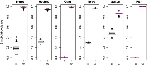
Figure 4 presents the simplicial deviances of the unweighted (U) and weighted (W) versions. The horizontal lines are the values for the original data, and the boxplots present the results of the 1000 bootstrapped tables. In all cases we can see a clear advantage of weighting, which allows to shift much more information to the interaction table.

6 Summary and Conclusions

CA is generally considered an exploratory data analysis tool. The method is motivated by an algorithm, and there is still a continuous discussion about its mathematical background; see, for example, Breitung [35]. The aim of this paper was to show that the link to the logratio methodology [36] as its limiting case, Greenacre [4] can contribute to build a solid theoretical framework for CA. We have shown that the unweighted LRA, which performs an SVD of the centered logratio represented compositions [4], is equivalent to an analysis of a compositional table. In the latter case, the whole table is considered a composition, and it is not treated as a sample of compositional data. Moreover, the orthogonal decomposition of a compositional table into its independent and interaction parts enables us to assess the explained variability not only within the interaction part (corresponding in the jargon of CA to contingency ratios) but also within the whole (logratio) correspondence table.

Compositional data, and also compositional (correspondence) tables as their two-factorial decomposition, are characterized by the property of scale invariance [8]. The possibility of approaching unweighted or weighted LRA with power transformation by different representations of the same contingency table (cf. Results 1 and 2 in Greenacre [4]) indicates that scale invariance in a truly compositional sense is not the main strength of CA. Weighting with compositional tables is achieved instead through a change of the reference measure in the respective Bayes space. This leads to the usual choice of weighting in CA with row and column (arithmetic) marginals to new insights, and to a natural increment of the explained variance within the whole table. On top of that, weighting with compositional tables is equivalent to the weighted CA.

The reformulation of CA using compositional tables also guarantees distributional equivalence for both the unweighted and the weighted case, while the unweighted CA so far lacked this feature. Clearly, the aggregation in distributional equivalence needs to be reformulated in terms of the geometric mean, as it is the case for the marginals in a compositional table, and in general as a measure of central tendency in a truly ratio-scale analysis; however, it is merely nothing but the usual aggregation in the log-scale, from the viewpoint of the original scale [16, 26]. Still, for the weighted case also the usual arithmetic marginals play the important role in providing the absolute (interval-scale) information, which is essentially their role in data analysis. Herewith, the benefits of both concepts of marginals can be utilized.

The whole concept can be easily extended to the case of -factors, , known under the name compositional cubes [37]. They represent the discrete version of the orthogonal decomposition of multivariate densities [16]. Due to the orthogonality of the decomposition, the explained variance of all possible combinations of factors can be assessed which is of particular importance in high-dimensional settings.

Of course, with the logratio approach, the problem of zeros naturally occurs, which needs to be carefully considered. The zeros in contingency tables can be, however, treated as so-called count zeros where a reasonable imputation by non-zero values is adequate, and approaches for this purpose are available [38]. Moreover, the effect of the imputation (and presence of zeros in general) is naturally downweighted in the weighted logratio CA by lowering the respective marginal values. Still, dealing with zeros in the logratio CA is one of the next challenges to be addressed.

Overall, the logratio approach to CA opens up many new potential avenues for how the field can be further developed. The R source codes for both weighted and unweighted CA using the compositional tables methodology and for the numerical experiments are available at https://github.com/kfacevicova.

Author Contributions

K.F., K.H., and P.F. contributed with theory, numerical experiments, and with paper writing.

Acknowledgments

K.H. and K.F. were supported by the Czech Science Foundation (grant 22-15684L) and the project ReDiKid: Resilient Kid in Digital World (reg. no. CZ.02.01.01/00/23_025/008686), co-funded by the European Commission. P.F. was supported by the Austrian Science Fund (grant DOI: 10.55776/I5799). Open access funding was provided by Technische Universität Wien/KEMÖ.

Conflicts of Interest

The authors declare no conflicts of interest.

Open Research

Data Availability Statement

Data sharing is not applicable to this article as no new data were created or analyzed in this study.

References

1J.-P. Benzécri, “ L'Analyse des Données,” in L'Analyse des Correspondances, vol. II (Dunod, 1973).
Google Scholar
2L. A. Goodman, “Measures, Models, and Graphical Displays in the Analysis of Cross-Classified Data,” Journal of the American Statistical Association 86, no. 416 (1991): 1085–1111.
10.1080/01621459.1991.10475155
Web of Science® Google Scholar
3M. Greenacre, Correspondence Analysis in Practice (Chapman & Hall/CRC, 2017).
10.1201/9781315369983
Google Scholar
4M. Greenacre, “Log-Ratio Analysis Is a Limiting Case of Correspondence Analysis,” Mathematical Geosciences 42 (2010): 129–134.
10.1007/s11004-008-9212-2
Web of Science® Google Scholar
5G. Box and D. Cox, “An Analysis of Transformations (With Discussion),” Journal of the Royas Statistical Society, Series B 35 (1964): 473–479.
Google Scholar
6J. Aitchison, The Statistical Analysis of Compositional Data (Chapman & Hall, 1986).
10.1007/978-94-009-4109-0
Google Scholar
7J. Aitchison and M. Greenacre, “Biplots of Compositional Data,” Journal of the Royal Statistical Society: Series C: Applied Statistics 51, no. 4 (2002): 375–392.
10.1111/1467-9876.00275
Web of Science® Google Scholar
8V. Pawlowsky-Glahn, J. Egozcue, and R. Tolosana-Delgado, Modeling and Analysis of Compositional Data (Wiley, 2015).
10.1002/9781119003144
Google Scholar
9M. Greenacre, Compositional Data Analysis in Practice (CRC Press, 2018).
10.1201/9780429455537
Google Scholar
10P. Filzmoser, K. Hron, and M. Templ, Applied Compositional Data Analysis (Springer, 2018).
10.1007/978-3-319-96422-5
Google Scholar
11J. Egozcue, V. Pawlovsky, M. Templ, and K. Hron, “Independence in Contingency Tables Using Simplicial Geometry,” Communications in Statistics 44, no. 18 (2015): 3978–3996.
10.1080/03610926.2013.824980
Google Scholar
12J. J. Egozcue, J. L. Díaz-Barrero, and V. Pawlowsky-Glahn, “ Compositional Analysis of Bivariate Discrete Probabilities,” in Proceedings of CODAWORK'08, the 3rd Compositional Data Analysis Workshop, ed. J. Daunis-i-Estadella and J. Martín-Fernández (University of Girona, 2008).
Google Scholar
13K. Fačevicová, K. Hron, V. Todorov, and M. Templ, “General Approach to Coordinate Representation of Compositional Tables,” Scandinavian Journal of Statistics 45, no. 4 (2018): 879–899.
10.1111/sjos.12326
Web of Science® Google Scholar
14M. Greenacre, “The Chipower Transformation: A Valid Alternative to Logratio Transformations in Compositional Data Analysis,” Advances in Data Analysis and Classification 18 (2024): 769–796.
10.1007/s11634-024-00600-x
Web of Science® Google Scholar
15M. Greenacre and P. Lewi, “Distributional Equivalence and Subcompositional Coherence in the Analysis of Compositional Data, Contingency Tables and Ratio-Scale Measurements,” Journal of Classification 26 (2009): 29–54.
10.1007/s00357-009-9027-y
Web of Science® Google Scholar
16C. Genest, K. Hron, and J. Nešlehová, “Orthogonal Decomposition of Multivariate Densities in Bayes Spaces and Relation With Their Copula-Based Representation,” Journal of Multivariate Analysis 198 (2023): 105228.
10.1016/j.jmva.2023.105228
Web of Science® Google Scholar
17J. de Sousa, K. Hron, K. Fačevicová, and P. Filzmoser, “Robust Principal Component Analysis for Compositional Tables,” Journal of Applied Statistics 48, no. 2 (2021): 214–233.
10.1080/02664763.2020.1722078
PubMed Google Scholar
18A. D'Ambra, G. Meccariello, and L. Della Ragione, “Weighted Cumulative Correspondence Analysis Based on a Particular Cumulative Power Divergence Family,” Annals of Operations Research 342 (2024): 1407–1428.
10.1007/s10479-022-04718-z
Web of Science® Google Scholar
19K. Hron, A. Menafoglio, J. Palarea-Albaladejo, P. Filzmoser, R. Talská, and J. Egozcue, “Weighting of Parts in Compositional Data Analysis: Advances and Applications,” Mathematical Geosciences 54 (2022): 71–93.
10.1007/s11004-021-09952-y
Web of Science® Google Scholar
20V. Choulakian, Scale Invariant Correspondence Analysis (IEEE, 2023).
Google Scholar
21P. Lewi, “Spectral Mapping, a Technique for Classifying Biological Activity Profiles of Chemical Compounds,” Arzneimittel-Forschung/Drug Research 26, no. 7 (1976): 1295–1300.
CAS PubMed Web of Science® Google Scholar
22J. J. Egozcue, J. L. Díaz-Barrero, and V. Pawlowsky-Glahn, “Hilbert Space of Probability Density Functions Based on Aitchison Geometry,” Acta Mathematica Sinica 22, no. 4 (2006): 1175–1182.
10.1007/s10114-005-0678-2
Web of Science® Google Scholar
23K. van den Boogaart, J. Egozcue, and V. Pawlowsky-Glahn, “Bayes Hilbert Spaces,” Australian & New Zealand Journal of Statistics 56, no. 2 (2014): 171–194, https://doi.org/10.1111/anzs.12074.
10.1111/anzs.12074
Web of Science® Google Scholar
24R. Talská, A. Menafoglio, K. Hron, J. Egozcue, and J. Palarea-Albaladejo, “Weighting the Domain of Probability Densities in Functional Data Analysis,” Statistics in Medicine 9, no. 1 (2020): e283.
10.1002/sta4.283
Google Scholar
25V. Choulakian, J. de Tibeiro, and P. Sarnacchiaro, “On the Choice of Weights in Aggregate Compositional Data Analysis,” Behaviormetrika (2024), https://doi.org/10.1007/s41237-024-00234-5.
10.1007/s41237-024-00234-5
Google Scholar
26G. Mateu-Figueras and V. Pawlowsky-Glahn, “A Critical Approach to Probability Laws in Geochemistry,” Mathematical Geosciences 40 (2008): 489–502.
10.1007/s11004-008-9169-1
Web of Science® Google Scholar
27J. McChesney, “You Should Summarize Data With the Geometric Mean,” 2016, https://jlmc.medium.com/understanding-three-simple-statistics-for-data-visualizations-2619dbb3677a.
Google Scholar
28J. Egozcue and V. Pawlowsky-Glahn, “Groups of Parts and Their Balances in Compositional Data Analysis,” Mathematical Geology 37, no. 7 (2005): 795–828.
10.1007/s11004-005-7381-9
Web of Science® Google Scholar
29R. Björck and G. H. Golub, “Numerical Methods for Computing Angles Between Linear Subspaces,” Mathematics of Computation 27, no. 123 (1973): 579–594.
10.1090/S0025-5718-1973-0348991-3
Web of Science® Google Scholar
30T. Reynkens, “rospca: Robust Sparse PCA Using the ROSPCA Algorithm,” R Package Version 1.0.4, 2018.
Google Scholar
31M. Greenacre, “Correspondence Analysis of the Spanish National Health Survey,” Gaceta Sanitaria 16 (2002): 160–170.
10.1016/S0213-9111(02)71648-8
CAS PubMed Google Scholar
32J. Martín-Fernández, C. Barceló-Vidal, and V. Pawlowsky-Glahn, “Dealing With Zeros and Missing Values in Compositional Data Sets Using Nonparametric Imputation,” Mathematical Geology 35, no. 3 (2003): 253–278.
10.1023/A:1023866030544
Web of Science® Google Scholar
33F. Galton, “Regression Towards Mediocrity in Hereditary Stature,” Journal of the Anthropological Institute of Great Britain and Ireland 15 (1886): 246–263.
10.2307/2841583
Google Scholar
34C. Cuadras and M. Greenacre, “A Short History of Statistical Association: From Correlation to Correspondence Analysis to Copulas,” Journal of Multivariate Analysis 188 (2022): 104901.
10.1016/j.jmva.2021.104901
Web of Science® Google Scholar
35J. Breitung, “ Dr. Strangelove or How I Learned to Stop Worrying and Love Correspondence Analysis,” in Multivariate Scaling Methods and the Reconstruction of Social Spaces, ed. A. Barth, F. Leßke, R. Atakan, M. Schmidt, and Y. Scheit (Verlag Barbara Budrich, 2023).
10.2307/jj.7330043.5
Google Scholar
36J. Aitchison, “The Statistical Analysis of Compositional Data (With Discussion),” Journal of the Royal Statistical Society, Series B (Statistical Methodology) 44, no. 2 (1982): 139–177.
10.1111/j.2517-6161.1982.tb01195.x
Web of Science® Google Scholar
37K. Fačevicová, P. Filzmoser, and K. Hron, “Compositional Cubes: A New Concept for Multi-Factorial Compositions,” Statistical Papers 64 (2022): 955–985.
10.1007/s00362-022-01350-8
PubMed Web of Science® Google Scholar
38J. Martín-Fernández, K. Hron, M. Templ, P. Filzmoser, and J. Palarea-Albaladejo, “Bayesian-Multiplicative Treatment of Count Zeros in Compositional Data Sets,” Statistical Modelling 15, no. 2 (2015): 134–158.
10.1177/1471082X14535524
Web of Science® Google Scholar

Volume18, Issue4

August 2025

e70023

Correspondence Analysis From the Viewpoint of Compositional Tables

ABSTRACT

1 Introduction

2 Unweighted CA

2.1 Logratio Analysis (LRA)

2.2 Compositional Tables

2.3 CA of a Compositional Table

3 Generalization: Weighted CA

3.1 Weighted CA and LRA

3.2 Weighted CA of a Compositional Table

3.3 Choice of Weights and Implications

4 Distributional Equivalence of the Logratio Approach

5 Numerical Experiments

5.1 Bootstrapping Tables

5.2 Comparison by the Principal Angle

5.3 Spanish Health Survey Data

5.4 Further Data Sets

6 Summary and Conclusions

Author Contributions

Acknowledgments

Conflicts of Interest

Open Research

Data Availability Statement

References

Figures

References

Information

About Wiley Online Library

Help & Support

Opportunities

Connect with Wiley

Correspondence Analysis From the Viewpoint of Compositional Tables

ABSTRACT

1 Introduction

2 Unweighted CA

2.1 Logratio Analysis (LRA)

2.2 Compositional Tables

2.3 CA of a Compositional Table

3 Generalization: Weighted CA

3.1 Weighted CA and LRA

3.2 Weighted CA of a Compositional Table

3.3 Choice of Weights and Implications

4 Distributional Equivalence of the Logratio Approach

5 Numerical Experiments

5.1 Bootstrapping Tables

5.2 Comparison by the Principal Angle

5.3 Spanish Health Survey Data

5.4 Further Data Sets

6 Summary and Conclusions

Author Contributions

Acknowledgments

Conflicts of Interest

Open Research

Data Availability Statement

References

Figures

References

Related

Information