Large eddy simulation of the flow over a canopy with spanwise patches
Abstract
In the present contribution, a numerical simulation of the flow over idealized aquatic canopy patches is presented. These patches consist of flexible blades interacting with the surrounding flow. The physical parameters governing the flow, the characteristics of the blades and their positioning within the vegetation patches are identical to a previously studied homogeneous scenario where the monami phenomenon occurs. A recently developed own numerical method capable of representing such a situation is used to generate high resolution data for the turbulent flow and the motion of the individual structures. Analysis is carried out in comparison with the homogeneous reference case. It is found that the clearance between the patches introduces substantial streamwise variation in the statistical quantities of this turbulent flow.
1 MOTIVATION
Understanding of the hydrodynamics related to vegetated canopies is crucial for modeling and possibly preserving aquatic ecosystems and life within. Natural vegetation canopies generally occur in patches, formed by several dynamic processes, including interaction with flow currents and deposit of sediment [1-3]. The amount of data retrievable from field studies, for example, Refs. [4, 5], and laboratory experiments with artificial plants, for example, Refs. [6, 7] are limited by the reduced optical access within the canopy and the overall effort of three-dimensional measurements. Scale-resolving numerical simulations, on the other hand, provide very detailed data, but the presence of deformable plants poses additional challenges to already expensive scale-resolving numerical simulations. Regardless of the approach of investigation, simplified model configurations have been devised to reduce the number of relevant parameters. These include the use of dowel-like rigid model plants [8], the investigation of isolated, circular patches [9, 10], and entirely homogeneous situations [11].
While the latter are especially suited for numerical studies where periodic boundary conditions can easily enforce homogeneity, experimental investigations always face the difficulty of limited extents. However, the homogeneous case is expected to represent the situation at the core of a sufficiently large patch, if far enough from the patch edges, that is, when allowing for homogeneous canopy conditions to establish. This development length, , is identified as the length at which the mixing layer at the canopy top is fully developed, reflected by the condition , with h the average height of the deformed blades, as illustrated in Figure 1. Values for are reported in the range [8].
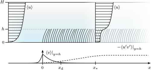
The present contribution discusses a case with spanwise patches repeating periodically along the streamwise direction. Each one of these patches is composed of regularly arranged flexible blades, setup according to the homogeneous canopy case studied by the present authors in Tschisgale et al. [11]. As such, the arrangement can also be seen as an infinite canopy featuring periodically reoccurring clearances extending in spanwise direction. Below, the simulation data are evaluated in comparison with the data of Tschisgale et al. [11].
2 PHYSICAL MODEL
The physical problem considered is sketched in the smaller insert of Figure 2. It consists of a flow of constant bulk velocity U, as driven by gravity, for example, over a set of patches infinitely long in spanwise direction and extension Lp in streamwise direction. Together with the clearing after the patch, the period in streamwise direction is . The floor is solid and flat. The free surface above the canopy at is also considered flat, to remove any wave effect.
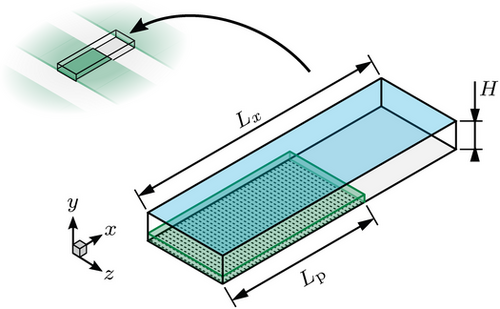
This setup is based on the homogeneous canopy simulation of Tschisgale et al. [11], which itself mimics the experiment of Okamoto and Nezu [6] where model vegetation was made up of strips of overhead projector film, placed in a water channel. These blades of length L were attached perpendicularly to the channel floor, facing the flow (see Figure 3 below), which is done here as well. Their fixations are laid out in a regular pattern with center-to-center distances of , both, in x and z. The definitions of the relevant parameters, as well as their values employed, are listed in Table 1. Resulting dimensionless numbers are given in Table 2. Expecting a mean deflection of the blades similar to the homogeneous case of in Tschisgale et al. [11] yields a relative patch length of .
| Variable | Value | ||
|---|---|---|---|
| Setup | U | Bulk velocity | |
| H | Channel height | ||
| Lp | Length of the canopy patch | ||
| Streamwise periodic length | |||
| g | Gravitational acceleration | ||
| Blade spacing in x and z | |||
| Fluid | ρ | Density | |
| ν | Kinematic viscosity | ||
| Structures | L | Length | |
| W | Width | ||
| T | Thickness | ||
| ρs | Density | ||
| E | Young's modulus |
| Definition | Value | |
|---|---|---|
| Bulk Reynolds number | ||
| Galilei number | ||
| 17 | Cauchy number | |
| −0.34 | Buoyancy number | |
| λ = | 0.55 | Unreconf. roughness density |
| −0.4 | Relative density difference | |
| 17.4 | Patch length ratio | |
| 3 | Unreconfigured submergence | |
| 0.013 | Blade cross-section asp. ratio |

3 NUMERICAL MODEL
Coupling between fluid and structure was established by the Immersed-Boundary Method of Tschisgale and Fröhlich [13], suitable for structures of vanishing thickness, and realizing a no-slip coupling condition. Further details of the method can be found in Refs. [11, 13]. Subgrid-scale turbulence was handled with the Large Eddy Simulation approach using the Smagorinsky model, with subgrid viscosity damped near the blades. Relevant numerical parameters are provided in Table 3.
| Variable | Value | |
|---|---|---|
| Spanwise extent | ||
| Ns | 760 | Blades in the patch |
| Ne | 30 | Segments per blade |
| Cells for fluid | ||
| Cell edge length | ||
| CS | 0.15 | Smagorinsky constant |
For fluid and structures periodic conditions in streamwise direction with a period equal to were imposed, modeling an infinitely long stretch in this direction. The same was done in spanwise direction. The period in z is and was chosen large enough for the spanwise two-point correlation to decay to zero [11], which is the usual requirement for this frequently applied approach. At the bottom wall, a no-slip condition was imposed, as well as on the blade surfaces. At the top wall, a symmetry condition was applied, equivalent to what is termed a rigid-lid condition in the community. Statistics were collected after an initial transient in the production simulation allowing for the flow (and the blade motion) to reach a developed stage.
4 RESULTS
4.1 Instantaneous flow
An impression of the flow is given in Figure 3, with all graphs generated for the same instant in time. Upon visual inspection of these instantaneous data (Figure 3), flow patterns above the canopy are, at first glance, overall comparable to those observed in Tschisgale et al. [11]. The monami phenomenon occurs, with deflected canopy sections accompanied by high-speed velocity streaks, and sometimes also Kelvin–Helmholtz (KH) type vortex structures. Streamwise instantaneous velocity shows patterns with angles of approximately 20° in x–y planes, as known from flat plate turbulent boundary layers [14]. Streaks of high and low streamwise velocity have widths in the order of H and are elongated in streamwise direction. They appear to be less likely populated by hairpin or KH-hairpin vortices than in the homogeneous reference case. This is attributed to the cavity, which affects the shear stress and hinders coherent structures from fully developing. KH vortex structures, in particular, tend to disintegrate behind the trailing canopy edge, while hairpin-like structures further away from the bottom seem more likely to survive into the next period. Overall, the situation appears less organized than in Tschisgale et al. [11, fig. 16], with the picture dominated by smaller-scaled, noisier vortex structures. As expected, the bottom wall shear magnitude is strongest adjacent to the canopy blades, with mean shear becoming weaker with increasing distance from the leading edge. Instantaneous wall shear is also elevated where blades are more deflected. In the cavity, striking patterns with lengthy streaks at scales comparable to the width of the blades appear. This observation still requires further analysis.
4.2 2D statistics
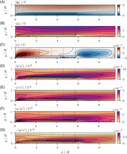
Field data were averaged in time, in the spanwise direction, and over a streamwise distance equal to the spacing of the blades, . The most important fields are shown in Figure 4. Obviously, the canopy acts as an obstacle, displacing streamlines upwards, and accelerating the flow above the canopy while decelerating the flow within. Consequently, there is an updraft behind the leading edge, and a downdraft behind the trailing edge. In a small region immediately behind the last rows around , the flow tends upwards as well, reminiscent of the recirculation behind a backward facing step. Turbulence intensity is strongest slightly above the canopy top, with the streamwise contribution dominating. Notable is also the region behind the leading edge where elevated Reynolds stresses are recognized.
4.3 Vertical profiles and comparison to homogeneous case
For comparison with the homogeneous reference case, profiles were extracted at the six equally spaced locations marked by dotted lines in Figure 4. They range from the point of fixation of the first structure to that of the last structure downstream. The resulting profiles are shown in Figure 5 together with those for the homogeneous reference case.

Starting from the leading edge, the homogeneous velocity profile is reached rather fast, while all other profiles remain significantly below the reference profiles, highlighting that the canopy length would not be sufficient to conclude on homogeneous flow characteristics at any location. This assessment is also corroborated by the development of statistics with x shown in Figure 6. These include fluid statistics extracted at the homogeneous canopy height of Tschisgale et al. [11], hhom, wall shear, and statistics of the blade tips. While the vertical velocity component does approach zero, similar to the trend sketched in Figure 1, it does so only towards the end of the patch, where a downdraft is promoted by the trailing flow, anyway. In addition, the main shear Reynolds stress component keeps climbing until the end of the patch, such that the development length is not reached. Overall, the mean flow introduces vertical transport of momentum and scalars, should they be present. The turbulent shear stress, , however, remains substantially below the developed profile above the canopy, as well as the vertical fluctuations .
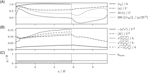
Figure 6 also contains information about the motion of the blades, with and representing the streamwise and vertical position of the tips, respectively. The amplitudes vary by 20% to 50% from the leading edge to the trailing edge. The vertical fluctuations remain smaller than the streamwise ones since the blades remain fairly erect. The fact that remains between the two demonstrates that and behave synchronously. This supports that the blades deform dominantly in first-order bending mode, as in Tschisgale et al. [11].
5 CONCLUSIONS
The present paper shows how the introduction of clearances into an otherwise homogeneous canopy alters the statistics of fluid and blades. The streamwise period chosen is below the one where a developed state would eventually be reached. Furthermore, the gap is small enough to create an impact of the trailing edge flow on the subsequent leading edge. Hence, this creates a new feature beyond leading edge effect and trailing edge recovery. Further simulations were conducted with a smaller value of , but are not reported here for lack of space.
ACKNOWLEDGMENTS
This work was funded by the French-German ANR-DFG project ESCaFlex (Agence Nationale de la Recherche, grant ANR-16-CE92-0020; Deutsche Forschungsgemeinschaft, grant 634058). The authors are also grateful to the Center for Information Services and High Performance Computing (ZIH) at TU Dresden for providing its facilities for high throughput calculations.
Open access funding enabled and organized by Projekt DEAL.


