Volume 23, Issue 4 e202300160
RESEARCH ARTICLE
Open Access

Isogeometric cohesive zone modeling of interfaces in reinforced concrete structures

Simon Klarmann

Simon Klarmann

Lehrstuhl für Baustatik und Baudynamik, RWTH Aachen University, Aachen, Germany

Search for more papers by this author
Georgia Kikis

Georgia Kikis

Lehrstuhl für Baustatik und Baudynamik, RWTH Aachen University, Aachen, Germany

Search for more papers by this author
Sven Klinkel

Corresponding Author

Sven Klinkel

Lehrstuhl für Baustatik und Baudynamik, RWTH Aachen University, Aachen, Germany

Correspondence

Sven Klinkel, Lehrstuhl für Baustatik und Baudynamik, RWTH Aachen, Mies-van-der-Rohe-Str. 1, 52074 Aachen, Germany.

Email: [email protected]

Search for more papers by this author
Rostislav Chudoba

Rostislav Chudoba

Lehrstuhl und Institut für Massivbau, RWTH Aachen University, Aachen, Germany

Search for more papers by this author
First published: 26 October 2023

Abstract

In reinforced concrete structures, the correct representation of the bond between concrete and reinforcement is a challenging task, since different mechanisms are acting simultaneously. On the other hand, the exact description of the reinforcement's geometry is not sufficient when using Lagrange shape functions and can additionally alter the modeling of this interaction. Isogeometric analysis enables the exact representation of complex geometries, and thus, can improve the correct description of the interface mechanisms. The concrete matrix and the reinforcement are modeled using boundary representation together with Non-Uniform Rational B-Spline (NURBS) and B-splines Scaled Boundary Isogeometric Analysis (SBIGA) which is in accordance with the modeling technique in Computer Aided Design (CAD) tools. This allows for a straightforward use of the design model in the analysis process. The interaction mechanisms between reinforcement and concrete are modeled using a zero-thickness interface in combination with a thermodynamically consistent cohesive zone model that captures the decohesion, compression and sliding effects. It includes a coupled damage-plasticity dissipation for the normal and tangential direction. The model is verified using experimental results and a comparison to the standard finite element method (FEM) is carried out in order to investigate the benefits of applying isogeometric analysis for the exact representation of the reinforcement.

1 INTRODUCTION

In the interface region between the concrete matrix and reinforcement, different mechanisms are acting that also influence one another, thus, making the correct description of the bond behavior difficult. At the same time, the use of Lagrange shape functions to describe circular or elliptical geometries, as it is common for reinforcement like steel bars, leads to higher computational cost and lower accuracy. Furthermore, since the mechanisms of the interface depend on the contact area between the concrete matrix and the reinforcement, the use of an approximation of the area instead of the exact value influences the bond behavior. In the past, cohesive zone elements have been combined with isogeometric analysis in order to take advantage of the higher continuity of NURBS basis functions [1, 2]. Furthermore, isogeometric analysis allows for the use of the exact geometry in the analysis process. Since CAD tools use a boundary representation modeling technique, that is, the solid is described solely by the boundary surfaces of the solid, the description of the concrete and reinforcement using the scaled boundary method is advantageous. Here, the cohesive zone model from Chudoba et al. [3] is combined with isogeometric analysis in order to capture the exact geometry of the interface between the concrete and reinforcement and thus, the bond behavior between these two materials. The concrete matrix and reinforcement is modeled using the Scaled Boundary Isogeometric Analysis (SBIGA).

2 PARAMETRIZATION OF SOLIDS USING SBIGA
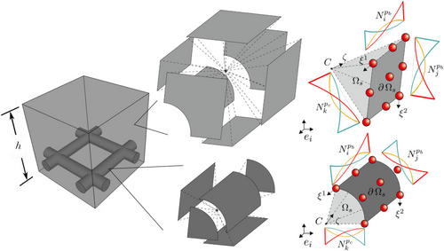
The SBIGA, which is a combination of the scaled boundary representation and isogeometric analysis [4], is used for the description of the concrete and reinforcement. In this approach, a 3D solid is described by its boundary surfaces that are scaled starting from the scaling center and along the scaling direction. This is in accordance with the boundary representation modeling technique used in CAD tools and allows for a direct use of the exact geometry in the analysis process. Furthermore, due to the higher continuity of splines, curved geometries, which are common for reinforcement, can be described with less computational effort. In SBIGA the solid is divided into sections and parameterized using two boundary surface parameters ξ α $\xi ^{\alpha }$ with α { 1 , 2 } $\alpha \in \lbrace 1,2 \rbrace$ and one scaling parameter 0 ζ 1 $0\le \zeta \le 1$ . The displacements are approximated as follows
u ( ξ 1 , ξ 2 , ζ ) = N b ( ξ 1 , ξ 2 ) N c ( ζ ) U = N U $$\begin{align} \bm{u}(\xi ^1,\xi ^2,\zeta )=\bm{N}_b(\xi ^1,\xi ^2)\bm{N}_c(\zeta )\bm{U}=\bm{N}\bm{U} \end{align}$$ (1)
where U includes the degrees of freedom of all control points of the corresponding section. N c ( ζ ) $\bm{N}_c(\zeta )$ contains the uni-variate B-spline basis functions of the scaling direction while N b ( ξ 1 , ξ 2 ) $\bm{N}_b(\xi ^1,\xi ^2)$ includes the NURBS basis functions R I $R_I$ that are used for the description of the boundary surfaces
N b ( ξ 1 , ξ 2 ) = R 1 0 0 R 2 0 0 R n b s 0 0 0 R 1 0 0 R 2 0 0 R n b s 0 0 0 R 1 0 0 R 2 0 0 R n b s $$\begin{align} \bm{N}_b(\xi ^1,\xi ^2)={\left[ \begin{matrix} R_1 & 0 & 0 & R_2 & 0 & 0 & \dots & R_{n_{bs}} & 0 & 0\\ 0 & R_1 & 0 & 0 & R_2 & 0 & \dots & 0 & R_{n_{bs}} & 0\\ 0 & 0 & R_1 & 0 & 0 & R_2 & \dots & 0 & 0 & R_{n_{bs}} \end{matrix}\right]} \end{align}$$ (2)
The NURBS basis functions R I $R_I$ are defined with the help of the B-spline basis functions N i p b $N_i^{p_b}$ , N j p b $N_j^{p_b}$ as follows
R I ( ξ 1 , ξ 2 ) = N i p b ( ξ 1 ) N j p b ( ξ 2 ) w i j l = 1 n i m = 1 n j N l p b ( ξ 1 ) N m p b ( ξ 2 ) w l m $$\begin{align} R_I(\xi ^1,\xi ^2)=\dfrac{N_i^{p_b}(\xi ^1)N_j^{p_b}(\xi ^2)w_{ij}}{\displaystyle \sum _{l=1}^{n_i}\displaystyle \sum _{m=1}^{n_j} N_l^{p_b}(\xi ^1)N_m^{p_b}(\xi ^2)w_{lm}} \end{align}$$ (3)
where n i $n_i$ , n j $n_j$ the number of control points in the two surface directions, p b $p_b$ the polynomial degree of the NURBS basis functions and w i j $w_{ij}$ the weight factor. In Figure 1 the SBIGA approach is depicted for the case of a reinforced concrete cube.
Details are in the caption following the image
SBIGA concept applied for a reinforced concrete cube. At the right the “exploded view” of the reinforcement and concrete geometries with the corresponding control points in red and basis functions is depicted. SBIGA, scaled boundary isogeometric analysis.
In the context of SBIGA the discretized weak form of equilibrium is defined as
G ( u , δ u ) = s = 1 n s e c δ U T Ω s B T F ̂ T S d V Ω s N T b d V t Ω s N T t ¯ d A $$\begin{align} G(\bm{u},\delta \bm{u})=\sum _{s=1}^{n_{sec}}\delta \bm{U}^T{\left(\int _{\Omega _s}\bm{B}^T\hat{\bm{F}}^T\bm{S}\,\text{d}V-\int _{\Omega _s}\bm{N}^T\bm{b}\,\text{d}V-\int _{\partial _t\Omega _s}\bm{N}^T\bar{\bm{t}}\,\text{d}A\right)} \end{align}$$ (4)
where n s e c $n_{sec}$ is the number of sections, Ω s $\Omega _s$ is the volume of section s, b is the body force and t ¯ $\bar{\bm{t}}$ the boundary traction. S denotes the second Piola–Kirchhoff stress, matrix B is used for the interpolation of the gradient of the virtual displacement while matrix F ̂ $\hat{\bm{F}}$ contains the components of the deformation gradient, see ref. [4]. It should be noted that even though the formulation here is expressed using the second Piola–Kirchhoff stress, and by this extend the Green–Lagrange strains, in the following examples only small strains were considered.

3 ISOGEOMETRIC COHESIVE ZONE MODEL

The interface between the concrete and the reinforcement is described by an isogeometric cohesive zone model.

3.1 Parametrization and kinematics

The interface is modeled using an isogeometric solid with a minimal thickness ( t 0 $t\rightarrow 0$ ). The contact surfaces, here called upper and lower surface, are described with the same NURBS basis functions N b ( ξ 1 , ξ 2 ) $\bm{N}_b(\xi ^1,\xi ^2)$ as in Equation (2) while in the thickness direction linear basis functions are considered with only two control points, see Figure 2A. This way, the displacements of the upper and the lower surface are described as follows
u u ( ξ 1 , ξ 2 ) = N b ( ξ 1 , ξ 2 ) U b u $$\begin{align} \bm{u}^u(\xi ^1,\xi ^2)&=\bm{N}_b(\xi ^1,\xi ^2)\bm{U}_b^u \end{align}$$ (5)
u l ( ξ 1 , ξ 2 ) = N b ( ξ 1 , ξ 2 ) U b l $$\begin{align} \bm{u}^l(\xi ^1,\xi ^2)&=\bm{N}_b(\xi ^1,\xi ^2)\bm{U}_b^l \end{align}$$ (6)
where U b u $\bm{U}_b^u$ includes the three displacements of all control points of the upper surface and U b l $\bm{U}_b^l$ includes the three displacements of all control points of the lower surface. The covariant basis vectors of the surfaces are defined as
G α = X ξ α G 3 = N $$\begin{align} \bm{G}_{\alpha }=\dfrac{\partial \bm{X}}{\partial \xi ^{\alpha }} \hspace{45.0pt} \bm{G}_3=\bm{N} \end{align}$$ (7)
where X the position vector and N the normal vector of the surface. In order to apply the cohesive zone model from ref. [3], the displacements at an arbitrary point on the upper and lower surface have to be described with respect to an orthonormal basis system. Thus, in addition to Gi with i { 1 , 2 , 3 } $i\in \lbrace 1,2,3\rbrace$ a local Cartesian basis system Ai has to be introduced. It is defined as the orthonormal basis system that is as close as possible to the covariant basis system Gi, see ref. [5] and Figure 2B. Its basis vectors are given as
A 1 = 2 2 A ¯ ξ 1 A ¯ ξ 2 A 2 = 2 2 A ¯ ξ 1 + A ¯ ξ 2 A 3 = N $$\begin{align} \bm{A}_{1}=\dfrac{\sqrt {2}}{2}{\left(\overline{\bm{A}}_{\xi ^1}-\overline{\bm{A}}_{\xi ^2}\right)} \hspace{45.0pt} \bm{A}_{2}=\dfrac{\sqrt {2}}{2}{\left(\overline{\bm{A}}_{\xi ^1}+\overline{\bm{A}}_{\xi ^2}\right)} \hspace{45.0pt} \bm{A}_3=\bm{N} \end{align}$$ (8)
with
A ¯ ξ 1 = 1 2 A ξ 1 + A ξ 2 | 1 2 A ξ 1 + A ξ 2 | A ¯ ξ 2 = N × A ¯ ξ 1 | N × A ¯ ξ 1 | and A ξ 1 = G 1 | G 1 | A ξ 2 = G 2 | G 2 | $$\begin{align} \overline{\bm{A}}_{\xi ^1}=\dfrac{\frac{1}{2}{\left(\bm{A}_{\xi ^1}+\bm{A}_{\xi ^2}\right)}}{|\frac{1}{2}{\left(\bm{A}_{\xi ^1}+\bm{A}_{\xi ^2}\right)}|} \hspace{25.0pt} \overline{\bm{A}}_{\xi ^2}=\dfrac{\bm{N}\times \overline{\bm{A}}_{\xi ^1}}{|\bm{N}\times \overline{\bm{A}}_{\xi ^1}|} \hspace{25.0pt}\text{and} \hspace{25.0pt} \bm{A}_{\xi ^1}=\dfrac{\bm{G}_1}{|\bm{G}_1|} \hspace{25.0pt} \bm{A}_{\xi ^2}=\dfrac{\bm{G}_2}{|\bm{G}_2|} \end{align}$$ (9)
To describe the interaction of the surface in the cohesive zone, the relative displacement field u = u u u l $\mathbf {u}=\mathbf {u}^{u}-\mathbf {u}^{l}$ is separated into the normal and tangential components
u N = u z , u T = u T x , u T y T , $$\begin{equation} u_{N}=u_{z},\qquad \mathbf {u}_{T}={\left[u_{Tx},\,u_{Ty}\right]}^{T}, \end{equation}$$ (10)
see Figure 2(C).
Details are in the caption following the image
(A) Isogeometric cohesive zone element, (B) covariant and local Cartesian basis systems, and (C) relative displacements between the upper and lower surface.

3.2 Material model

This subsection briefly describes the material law proposed by the authors in ref. [3] for the cohesive zone element. The stresses associated with the three relative displacements presented in the previous chapter read
σ N = σ z , σ T = σ T x , σ T y T . $$\begin{equation} \sigma _{N}=\sigma _{z},\qquad \bm{\sigma }_{T}={\left[\sigma _{Tx},\,\sigma _{Ty}\right]}^{T}. \end{equation}$$ (11)
To describe the inelastic behavior of the cohesive zone model, the following internal state variables E $\bm{\mathcal {E}}$ and associated thermodynamic forces S $\bm{\mathcal {S}}$ are introduced
E = u N p , ω N , u T p , ω T , z , α , S = σ N p , Y N , σ T p , Y T , Z , X . $$\begin{equation} \bm{\mathcal {E}}={\left[u_{N}^{p},\,\omega _{N},\,\mathbf {u}_{T}^{p},\,\omega _{T},\,z,\,\bm{\alpha }\right]},\qquad \bm{\mathcal {S}}={\left[\sigma _{N}^{p},\,Y_{N},\,\bm{\sigma }_{T}^{p},\,Y_{T},\,Z,\,\mathbf {X}\right]}. \end{equation}$$ (12)
The state variables of Equation (12) consist of the plastic displacements u N p $u_{N}^{p}$ , u T p $\mathbf {u}_{T}^{p}$ , and the damage variables ω N $\omega _{N}$ , ω T $\omega _{T}$ in the normal and tangential direction, respectively. Furthermore, the isotropic and kinematic hardening variables z and α are defined, for the tangential directions. The associated thermodynamical force are the plastic stresses in normal σ N p $\sigma _{N}^{p}$ and tangential directions σ T p $\bm{\sigma }_{T}^{p}$ , the energy release rates in normal Y N $Y_{N}$ and tangential directions Y T $Y_{T}$ , the isotropic hardening stress Z and the back stress X $\mathbf {X}$ .
To describe the behavior of the cohesive zone, the free energy is split into a normal and a tangential part
ρ ψ E = ρ ψ N E + ρ ψ T E . $$\begin{equation} \rho \,\psi {\left(\bm{\mathcal {E}}\right)}=\rho \,\psi _{N}{\left(\bm{\mathcal {E}}\right)}+\rho \,\psi _{T}{\left(\mathcal {E}\right)}. \end{equation}$$ (13)
The individual parts of Equation (13) are for the normal component
ρ ψ N u N , u N p , ω N = 1 2 1 H σ N ω N E N u N u N p 2 , $$\begin{equation} \rho \,\psi _{N}{\left(u_{N},\,u_{N}^{p},\,\omega _{N}\right)}=\dfrac{1}{2}{\left(1-H{\left(\sigma _{N}\right)}\omega _{N}\right)}E_{N}{\left(u_{N}-u_{N}^{p}\right)}^{2}, \end{equation}$$ (14)
and for the tangential component
ρ ψ T u T , u T p , ω T , z , α = 1 2 1 ω T E T u T u T p · u T u T p + 1 2 K z 2 + 1 2 γ α · α . $$\begin{equation} \rho \,\psi _{T}{\left(\mathbf {u}_{T},\,\mathbf {u}_{T}^{p},\,\omega _{T},\,z,\,\bm{\alpha }\right)}=\dfrac{1}{2}{\left(1-\omega _{T}\right)}E_{T}{\left[{\left(\mathbf {u}_{T}-\mathbf {u}_{T}^{p}\right)}\cdot {\left(\mathbf {u}_{T}-\mathbf {u}_{T}^{p}\right)}\right]}+\dfrac{1}{2}K\,z^{2}+\dfrac{1}{2}\gamma {\left(\bm{\alpha }\cdot \bm{\alpha }\right)}. \end{equation}$$ (15)
Within Equations (14) and (15), E N $E_{N}$ and E T $E_{T}$ are the stiffness in the normal and tangential directions, respectively. The damage in the normal direction is only active in case of tension, considered by the Heaviside function H ( σ N ) $H(\sigma _{N})$ . Compared to the normal part, the tangential part also includes isotropic hardening with the associated hardening modulus K and kinematic hardening with the associated hardening modulus γ.
For the complete description of the material model and the necessary material parameters, it is required to introduce the elastic domain and the flow potential. The elastic domain is defined by the threshold function given as
f lin x , y ; y ¯ , x 0 , m = y y ¯ + m x x 0 , f ell x , y ; x ¯ , y ¯ , x 0 , m = y 2 b 2 + x x 0 x c 2 a 2 c . $$\begin{equation} f_{\text{lin}}{\left(x,y;\bar{y},x_{0},m\right)}={\left|y\right|}-\bar{y}+m{\left(x-x_{0}\right)},\qquad f_{\text{ell}}{\left(x,y;\bar{x},\bar{y},x_{0},m\right)}=\sqrt {\dfrac{y^{2}}{b^{2}}+\dfrac{{\left(x-x_{0}-x_{c}\right)}^{2}}{a^{2}}}-c. \end{equation}$$ (16)
The necessary parameters for a smooth transition between the functions f lin $f_{\text{lin}}$ and f ell $f_{\text{ell}}$ are
a = y ¯ m x ̂ y ¯ 2 m x ̂ · x ̂ c , b = y ¯ m x ̂ y ¯ 2 m x ̂ · y ¯ c , c = y ¯ + m 2 x ̂ 2 2 m x ̂ + y ¯ , x c = m x ̂ 2 2 m x ̂ + y ¯ , x ̂ = x 0 x ¯ . $$\begin{equation} a=-\dfrac{\bar{y}-m\,\hat{x}}{\bar{y}-2\,m\,\hat{x}}\cdot \dfrac{\hat{x}}{c},\quad b=\dfrac{\bar{y}-m\hat{x}}{\sqrt {\bar{y}-2\,m\,\hat{x}}}\cdot \dfrac{\sqrt {\bar{y}}}{c},\quad c=\bar{y}+\dfrac{m^{2}\hat{x}^{2}}{2\,m\,\hat{x}+\bar{y}},\qquad x_{c}=-\dfrac{m\,\hat{x}^{2}}{2\,m\,\hat{x}+\bar{y}},\quad \hat{x}=x_{0}-\bar{x}. \end{equation}$$ (17)
By defining two sets of arguments
N t = x = σ N e f f , y = q T e f f , x ¯ = f t , y ¯ = f S + Z , x 0 = 0 N c = x = σ N e f f , y = q T e f f , x ¯ = f c , y ¯ = f S + m f c 0 + Z , x 0 = f c 0 $$\begin{align} \mathcal {N}^{t} & ={\left\lbrace x=\sigma _{N}^{eff},\,y=q_{T}^{eff},\,\bar{x}=f_{t},\,\bar{y}=f_{S}+Z,\,x_{0}=0\right\rbrace} \nonumber \\ \mathcal {N}^{c} & ={\left\lbrace x=-\sigma _{N}^{eff},\,y=q_{T}^{eff},\,\bar{x}=f_{c},\,\bar{y}=f_{S}+m\,f_{c0}+Z,\,x_{0}=f_{c0}\right\rbrace} \end{align}$$ (18)
with
σ N eff = σ N P 1 H σ N p ω N = E N u N u N p , σ T eff = σ T p 1 ω T = E T u T u T p , q T eff = σ T eff X · σ T eff X , $$\begin{equation} \sigma _{N}^{\text{eff}}=\dfrac{\sigma _{N}^{P}}{1-H{\left(\sigma _{N}^{p}\right)}\omega _{N}}=E_{N}{\left(u_{N}-u_{N}^{p}\right)},\,\bm{\sigma }_{T}^{\text{eff}}=\dfrac{\bm{\sigma }_{T}^{p}}{1-\omega _{T}}=E_{T}{\left(\mathbf {u}_{T}-\mathbf {u}_{T}^{p}\right)},\,q_{T}^{\text{eff}}=\sqrt {{\left(\bm{\sigma }_{T}^{\text{eff}}-\mathbf {X}\right)}\cdot {\left(\bm{\sigma }_{T}^{\text{eff}}-\mathbf {X}\right)}}, \end{equation}$$ (19)
the elastic domain finally reads
f S eff = f N t = f ell N t if T N t > 0 f N c = f ell N c if T N t > 0 f T = q T eff f S + Z + m σ N eff otherwise , T x , y ; x ¯ , y ¯ , x 0 = y ¯ x 0 x c x x c y . $$\begin{align} f{\left(\bm{\mathcal {S}}^{\text{eff}}\right)} & ={\begin{cases} f_{N}^{t}=f_{\text{ell}}{\left(\mathcal {N}^{t}\right)} & \text{if }\mathcal {T}{\left(\mathcal {N}^{t}\right)}>0\\ f_{N}^{c}=f_{\text{ell}}{\left(\mathcal {N}^{c}\right)} & \text{if }\mathcal {T}{\left(\mathcal {N}^{t}\right)}>0\\ f_{T}=q_{T}^{\text{eff}}-{\left(f_{S}+Z\right)}+m\,\sigma _{N}^{\text{eff}} & \text{otherwise} \end{cases}},\quad \mathcal {T}{\left(x,y;\bar{x},\bar{y},x_{0}\right)}=\dfrac{\bar{y}}{x_{0}-x_{c}}{\left(x-x_{c}\right)}-{\left|y\right|}. \end{align}$$ (20)
Herein, the newly introduced material parameters are the elastic shear stress limit f S $f_S$ , the compressive interface strength f c $f_c$ , the transition limit f c 0 $f_{c0}$ from f T $f_T$ to f N c $f_N^c$ . Lastly, the definition of the flow potential is required. It reads
φ E , S = f E , S + φ N E , S + φ T E , S $$\begin{align} \varphi {\left(\bm{\mathcal {E}},\bm{\mathcal {S}}\right)} & =f{\left(\bm{\mathcal {E}},\bm{\mathcal {S}}\right)}+\varphi _{N}{\left(\bm{\mathcal {E}},\bm{\mathcal {S}}\right)}+\varphi _{T}{\left(\bm{\mathcal {E}},\bm{\mathcal {S}}\right)}\end{align}$$ (21)
φ N E , S = 1 ω N c N S N r N + 1 Y N S N r N + 1 H σ N p , φ T E , S = 1 ω T c T S T r T + 1 Y T S T r T + 1 . $$\begin{align} \varphi _{N}{\left(\bm{\mathcal {E}},\bm{\mathcal {S}}\right)} & ={\left(1-\omega _{N}\right)}^{c_{N}}\dfrac{S_{N}}{r_{N}+1}{\left(\dfrac{Y_{N}}{S_{N}}\right)}^{r_{N}+1}H{\left(\sigma _{N}^{p}\right)},\qquad \varphi _{T}{\left(\bm{\mathcal {E}},\bm{\mathcal {S}}\right)}={\left(1-\omega _{T}\right)}^{c_{T}}\dfrac{S_{T}}{r_{T+1}}{\left(\dfrac{Y_{T}}{S_{T}}\right)}^{r_{T}+1}. \end{align}$$ (22)
The flow potential (22) defines the necessary material parameters, which control the damage evolution. These are the damage accumulation exponents c N $c_N$ and c T $c_T$ , the damage rate exponents r N $r_N$ and r T $r_T$ , and the damage energy rate scaling parameters S N $S_N$ and S T $S_T$ in the normal and tangential directions, respectively. With the flow potential, the evolution equations of the internal variables are given as
Φ E , S = Υ φ E , S S E , E ̇ = λ Φ E , S , Υ = 1 , 1 , 1 , 1 , 1 , 1 . $$\begin{equation} \bm{\Phi }{\left(\bm{\mathcal {E}},\bm{\mathcal {S}}\right)}=-\varUpsilon \dfrac{\partial \varphi {\left(\bm{\mathcal {E}},\bm{\mathcal {S}}\right)}}{\partial \bm{\mathcal {S}}{\left(\bm{\mathcal {E}}\right)}},\qquad \dot{\bm{\mathcal {E}}}=\lambda \bm{\Phi }{\left(\bm{\mathcal {E}},\bm{\mathcal {S}}\right)},\qquad \varUpsilon ={\left[-1,\,-1,\,-1,\,-1,\,1,\,1\right]}. \end{equation}$$ (23)
The evolution equations Equation (23) are solved employing the backward Euler method.

4 NUMERICAL EXAMPLES

The numerical examples are used to demonstrated the capabilities of the material model.

4.1 Pull-out test

The pull-out test is intended as a first comparison of the finite element and Isogeometric Analysis (IGA) implementation of the cohesive element.

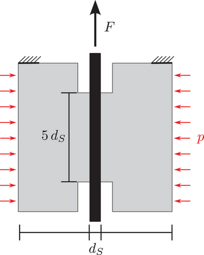
In Figure 3, the test setup is depicted. Herein, the steel bar is embedded in a concrete block. The diameter of the steel bar is d S = 16 $d_S=16$  (mm) and the contact length to the concrete is 5 d S $5\; d_S$ . For both, the concrete and steel material a linear elastic behavior is assumed. With a Young's modulus and Poisson ration of E S = 210 $E_S=210$ (GPa), ν S = 0.3 $\nu _S=0.3$ for the steel and E C = 31.7 $E_C=31.7$ (GPa), ν C = 0.221 $\nu _C=0.221$ for the concrete, respectively. For the cohesive element, the material parameters in tangential direction are: E T = 80 $E_T=80$ (MPa/mm), shear stress limit f S = 0.4 $f_S=0.4$ (MPa), damage energy rate scaling parameter S T = 0.0006 $S_T=0.0006$ (N/mm), damage rate exponent r T = 1 $r_T=1$ (-), damage accumulation exponent c T = 2.8 $c_T=2.8$ (-), isotropic hardening modulus K = 0 $K=0$ (MPa/mm), kinematic hardening modulus γ = 0 $\gamma =0$ (MPa/mm). In normal direction, the material parameters are: E N = 250 $E_N=250$ (MPa/mm), tensile interface strength f t = 0.2 $f_t=0.2$ (MPa), compressive interface strength f c = 40 $f_c=40$ (MPa) and f c 0 = 30 $f_{c0}=30$ (MPa), damage energy rate scaling parameter S N = 0.1 $S_N=0.1$ (N/mm), damage rate exponent r N = 1 $r_N=1$ (-), damage accumulation exponent c N = 1 $c_N=1$ (-). The pressure sensitivity parameter is m = 0.17 $m=0.17$ (-).

Details are in the caption following the image
System with loads.

As the test specimen is chosen such that there is barely any deformation in the concrete or the steel bar, the impact of refinement in the radial direction would not change the results. For the sake of completeness, the outer concrete is modeled with three elements in the radial direction for the Finite Element (FE) approximation, the inner concrete ring with three elements in the radial direction, and the steel bar with a three-by-three block and a surrounding lay to represent the circle. Eight elements are employed in the height direction, the area in which the steel is in contact with the concrete. For SBIGA, the outer concrete block and the steel bar were each divided into 16 patches with one element per patch, that is, eight elements in circumferential direction, two elements in height direction and one element in radial direction. The inner concrete ring was modeled using eight patches with one element per patch; thus, eight elements in circumferential direction, one element in height and radial direction.

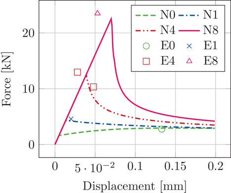
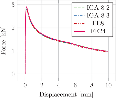
Figure 4 shows the good agreement of the IGA and FE results. In the case of IGA 8 2, with eight elements in circumferential direction of order 2, and IGA 8 3, with eight elements in circumferential direction of order 3, the results are almost identical and match with the FE results from FE8 and FE24 with 8 and 24 elements in the radial direction, respectively. This was expected, as the pull-out activates sliding in length direction of the steel bar. In this case, the IGA and FE models both approximate the geometric properties of the problem in the same way. To show the capabilities of the proposed material model, Figure 5 shows the comparison of the simulation results with the experimental data of ref. [6]. Herein, the lines are the load deflection curves of the numerical simulation and the marked points are the experimental data at the maximum loads of each individual test. The key point of this comparison is the applied pressure p to the system. The numbers indicate the pressure level: N0 means an applied pressure of p = 0 $p=0$ (MPa), N1 of p = 0.1 f c $p=0.1\;f_c$ , N4 of p = 0.4 f c $p=0.4\;f_c$ , and N8 p = 0.8 f c $p=0.8\;f_c$ . The N stand for the numerical simulation and E for the experimental data. In this case the analysis is performed on material level only.
Details are in the caption following the image
Pull-out test – results mesh refinement with FE.
Details are in the caption following the image
Pull-out test – comparison numerical results with experiments.

4.2 Torsion test

The torsion test is chosen to show the superiority of the IGA implementation of the cohesive element over the FE implementation. In this case, sliding is activated in the circumferential direction of the steel bar. As the material model is pressure dependent, only with an exact representation of the geometry, the converged results can be obtained.

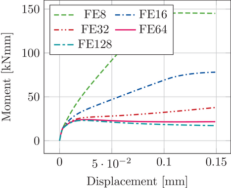
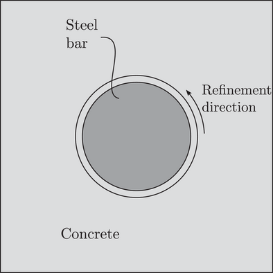
The model and material parameters are the same as in the pull-out test. Only the force F is replaced by a moment M. Figure 6 shows the top-view of the system with the refinement direction of the mesh. The results of the analysis with the FE implementation of the cohesive element are shown in Figure 7. Herein, the number of elements are indicated by the numbers in the names, for example, FE8 means eight elements in circumferential direction, FE16 means 16 elements in circumferential direction and so on. A convergent behavior can be observed, but very fine meshes are needed to obtain the correct results.
Details are in the caption following the image
System with loads.
Details are in the caption following the image
Torsion test – mesh refinement FE.

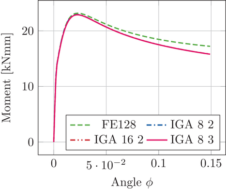
In contrast, Figure 8 shows the results of the IGA implementation of the cohesive element and compares it to the finest FE mesh (FE128). Herein, the IGA models are represented with two numbers, for example, IGA 8 2 which means eight elements in circumferential direction and an approximation order of 2 or IGA 8 3 which means eight elements in circumferential direction and an approximation order of 3 and so on. IGA 8 2 was chosen as the coarsest mesh since in SBIGA, every point of a patch has to be “visible” from the scaling center. In order to fulfill this for the inner concrete ring at least eight patches were necessary in circumferential direction. The results obtained by IGA are independent of mesh refinement and approximation order. Thus, in case of the proposed element very coarse meshes are sufficient to obtain the converged results when using IGA. Comparing the required number of equations, the IGA implementation of the cohesive element only requires 4202 equations, while the FE implementation requires 87 027 equations to get accurate results. Hence, the IGA implementation of the cohesive element is superior to the FE implementation. This example demonstrates the importance of an accurate geometry representation for the proposed material model because the results are strongly pressure dependent. Even if realistic reinforcements do not have a perfectly smooth surface, the accurate approximation drastically reduces the degrees of freedom.
Details are in the caption following the image
Torsion test – comparison FE with IGA.

5 CONCLUSIONS

In this work a cohesive zone model that considers decohesion, compression and sliding effects was combined with isogeometric analysis in order to accurately represent the bond between concrete and reinforcement. The concrete matrix and reinforcement were modeled using SBIGA, while the interface was described by an isogeometric solid element with zero thickness. The model was calibrated and validated using two examples. A comparison with the standard FEM showed that in the case were sliding occurs along the curved surface of the steel bar, the exact representation of the geometry using higher order NURBS basis functions leads to higher accuracy with less degrees of freedom. A comparison of the results from the simulation using the isogeometric cohesive zone element with experimental data from a pull-out test was made and showed good agreement. The calibration and validation of the model for carbon reinforced concrete structures within the framework of the Collaborative Research Center/Transregio 280 (SFB/TRR 280) is going to be the scope of future work. Furthermore, an incorporation of the isogeometric cohesive zone element into a FE 2 $\text{FE}^2$ scheme is planned.

ACKNOWLEDGMENTS

This research was funded by the Deutsche Forschungsgemeinschaft (DFG, German Research Foundation)–SFB/TRR 280. Projekt-ID: 417002380.

Open access funding enabled and organized by Projekt DEAL.

      The full text of this article hosted at iucr.org is unavailable due to technical difficulties.