1 INTRODUCTION

We are interested in discrete-time dynamical systems of the form

(1)

where is a matrix depending on a parameter μ chosen from an interval , is a noise term with , h is the time increment of the discretization, and stands for the matrix exponential function. We assume that is diagonalizable for all . We further assume that the dependency of A on μ is known, but the parameter μ itself is not. Estimating μ is the subject of this paper.

Discrete-time dynamical systems of the form (1) occur when applying the Euler–Maruyama method to solving a stochastic differential equation of the form

see, for instance, Kloeden and Platen [1] for details.

The paper focuses on the following example.

Example 1.1.Imagine we have a chain anchored below the water and on a pole above water. Submerged chain links are damped more than chain links in the air. The chain can be discretized by masses and springs like in Figure 1. We know the masses , the characteristics of the springs, and the damping when the masses are in the air as well as when they are in the water. However, we do not know the depth of the water μ or, if you like, how many of the masses are below water. The system is excited by external forces. We record the ensuing motion, that is we record the position of the masses at equidistant discrete time points, and try to infer the depth of water from said recording. Since the motion can be associated with the sound emitted one can arguably say that we are attempting to hear the depth of the water and hence the title of the paper.

Discretization leads to a matrix to describe this setup, where the parameter μ describes the depth of the water. We assume for simplicity that all masses are 1, that all spring characteristics are 1, and that the damping in water is 10, while the damping in air is 5. The mechanical system can be described with the second-order differential equation

(2)

where and 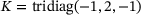. The matrix D is diagonal with a transition on the diagonal from 5 for the parts in the air to 10 for the parts in water. To make this transition smooth and to account for a reduced damping near the surface caused by waves, we use sigmoid-functions on the diagonal,

where n is the number of masses, that is . Equation (2) is a standard example of a quadratic eigenvalue problem that has been discussed in many publications, for instance in Refs. [2, 3]. We deliberately chose an overdamped system, that is one that fulfills

to ensure that all eigenvalues of are real and nonpositive [2, 4]. We linearize this quadratic eigenvalue problem to

Details on the linearization of quadratic eigenvalues can be found in the review paper [2].

In this paper, we pursue the following idea: A discretized trajectory of the noisy dynamical system (1) is recorded. This is combined with approximations of the functions describing the eigenvalues and eigenvectors of to estimate the most likely μ using a kernel density estimator. We choose a and use the 's for a coordinate transform to the eigenvector basis. We obtain new vectors describing the trajectory in the eigenbasis. If we have chosen the correct , then the components of decrease like with time . Obviously, as soon as the components become too small, the influence of the noise η becomes dominant. Thus even with the correct , the relation between and is not perfect. Nevertheless, each eigenpair i, each time step j, and each choice of provide an estimate for μ. We combine all these estimates by employing a kernel density estimator, which will provide us with the most likely guess of μ based on the individual guesses and a corresponding probability density, that is an uncertainty extimate. This is demonstrated by the numerical example in Section 4. Before we discuss the experiments, we provide a brief review in Section 2 regarding the computation of parametric eigenpairs of described in Mach and Freitag [5]. In Section 3, we discuss how μ is found.

2 TAYLOR SERIES AND CHEBYSHEV EXPANSIONS OF AND

Recently, Mach and Freitag presented a Taylor series and a Chebyshev expansion for the eigenvalue decomposition of , see Mach and Freitag [5] for details. They show how one can compute an approximation to the eigenvalues and eigenvectors,

First, a Taylor series is used for , , and about an expansion point μ₀. Under certain assumptions, the existence of such a series expansion for and is shown in Kato's book on perturbation theory for linear operators [6]. In particular, if is real and symmetric such a series converges. The idea of using Taylor series expansions for the perturbation analysis is not new and goes at least as far back as 1939 [7]. The Taylor coefficients regarding the expansion point μ₀ of v and λ can be successively computed by solving first

and then

Such linear systems have been used for first-order perturbation analysis, for instance, in Andrew et al. [8]. The novel contribution is the extension to use the same linear systems for the computation of higher-order derivatives for approximating the function and and the efficient implementation. In our numerical experiments, we are going to use the Matlab code provided by Mach [9]. In particular, if a Schur decomposition of A₀ is computed in the initial step, recall we need to solve anyway, then this Schur decomposition can be used to transform

see Mach and Freitag [5] for further details. The Schur decomposition can be computed with Francis's implicitly shifted QR algorithm in about [10-12]. The algorithm is described in many textbooks, among others in Aurentz et al. [13]. This enables us to compute the first p Taylor series coefficient for all eigenpairs in .

For the Chebyshev expansion, the algorithm is more complicated. Mach and Freitag used Chebyshev polynomials of second kind defined by

This has the consequence that for (follows with induction from Benjamin and Walton [14, Identity 3])

This minor difference to the monomial basis, for which holds, means that the Chebyshev coefficients cannot be computed one-by-one as for the Taylor series coefficients, but have to be computed all at once. Nonetheless, approximating the products with allows to use an approach similar to the Taylor polynomials to compute an initial approximation. Despite this rough approximation, the resulting eigenpairs are often accurate to three or four digits and serve as suitable starting points for a refinement with Newton's method, see Mach and Freitag [5] for further details. We observe that often the initial approximation places us within the area of quadratic convergence of Newton's method. Thus, three or four Newton steps often suffice to reach convergence to double precision.

Despite the increased costs, the Chebyshev expansion is preferable, due to the advantage of achieving a high approximation quality relatively homogeneously over the expansion interval. However, we observe a slight increase of the approximation error near the endpoints of the interval. The Taylor series approximation, by contrast, is mainly accurate near the expansion point μ₀ and looses accuracy with increased distance from μ₀. Thus, the numerical experiments in this paper solely use the Chebyshev expansion.

3 FINDING THE UNKNOWN PARAMETER μ

In this section, we discuss how μ can be found with the help of a trajectory and the eigenpairs of .

We perform a coordinate transform of trajectory onto the eigenbasis. That is, we compute

where is an initial guess for μ. Initially, we use equispaced in the interval of interest. Other choices based on a prior distribution are possible and are subject to future research. This coordinate transformation depends on . Hence, we fix a in the superscript. For , we have (see, for instance, Higham [15])

For the hidden , the components of evolve like an exponential function,

with the representation of η in the eigenbasis for . For other μ, the decay exponentially as well, but the effect is a mix of different . Ignoring , we have

We have made two simplifications and approximations: (1) We ignore the noise term η. This is justified since for large absolute values of , the η term is negligible. If the system is close to being stationary, the noise becomes very relevant and a more elaborate approach for inferring μ is needed. (2) We also ignore that for different , the eigenbasis changes. We are going to use both simplifications and will demonstrate that the results are useful despite of them.

We have an approximation . Thus, the polynomial 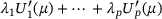approximates . We use this together with the difference between the quotient and the exponential of the eigenvalue to μ to guess μ by

(3)

This equation  is based on the linear Taylor polynomial:

We then solve for that μ which minimizes the difference between and .

For each combination of , , and we get a new guess of μ.1 We combine all of the guesses inside our interval of interest using Matlab's kernel density estimator ksdensity. This function computes for selected ξ the following sum:

where β is a predetermined bandwidth, essentially a parameter deciding how far is smoothed out, and where

is the kernel—a Gaussian kernel—used for the smoothing. As a result, we obtain a discretization of the density function with 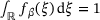. We pick the mode with

which is the most likely μ with respect to the probability density function.

Alternatively, one can use the density function to draw a new set of guesses based on the new distribution. This process can be iterated, see Section 5.

4 NUMERICAL EXPERIMENTS

This section is devoted to numerical experiments based on Example 1.1. For our numerical experiments, we use Matlab (R2020b) with IEEE 754 double precision arithmetic and a computer with Ubuntu 18.04.6 LTS, an Intel Core i7-10710U CPU (six physical cores), and 16 GB of RAM.

We first demonstrate the accuracy of the Chebyshev expansion approach by repeating some experiments from Mach and Freitag [5] with the matrix from Example 1.1. In Figure 2, we observe that a fourth-degree Chebyshev expansion with three Newton steps (solid blue line —) is sufficient to approximate the sampled eigenvalues (red crosses +) visually very well on the interval [2,4] and reasonably well outside the interval of interest. The visual impression of a small error is confirmed by the absolute error plot, see Figure 3.

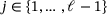
Our penultimate experiment is a demonstration that we can find a good approximation to a hidden μ. Figure 4 depicts the results. We use one trajectory with 50 time steps of size 1/10 each. The chosen starting point x₀ is randomly computed by 10*randn(20,1) and the added noise is computed by 1e-5*randn(20,1). We use a Chebyshev expansion up to degree 9 for the eigenvalues of Example 1.1 with 10 masses, that is . The interval of interest is [2,4] in which we use 15 equidistant-spaced to compute guesses for μ, see Figure 5 for the contribution of each to the density. The kernel density estimator indicates that the most likely μ is , while the actual μ used for the simulation of the trajectory was 3.2. This demonstrates that the described procedure is capable of inferring a good approximation of μ based on the parametric eigenpairs of .

5 CONCLUSIONS AND FUTURE WORK

We have successfully demonstrated that we can estimate the depth μ based on a recorded trajectory, that is recording the sound emitted by the mass-spring system is sufficient to hear the depth of the water. The necessary computations were aided by initially computing a parametric eigendecomposition of .

The guess of depends on the initial guess of μ. In the last section, we used 15 equidistant-spaced points in [2,4]. Using more points improves the accuracy and so does using points closer to the sought μ. Preliminary experiments reported in Figure 6 indicate that it is promising to draw new guesses for μ based on the estimated density and repeat the process with those. Beginning with the second iteration, we use 60 guesses for μ, which are shown as red crosses. We observe that the red crosses cluster closer and closer to the hidden . Figure 6 indicates the density function that seem to converge toward a delta-pulse at , see also Table 1. In the case of Table 1 the mode, the most likely μ, is a superior guess compared with the mean. These experiments are preliminary, since we observed different behavior for other examples. Once these differences are fully understood, we will report these experiments elsewhere. Other future work may involve investigations into the dependency on the noise level and extensions to 2 or more parameters.