Monte Carlo tree search for dynamic shortest-path interdiction
Abstract
We present a reinforcement learning-based heuristic for a two-player interdiction game called the dynamic shortest path interdiction problem (DSPI). The DSPI involves an evader and an interdictor who take turns in the problem, with the interdictor selecting a set of arcs to attack and the evader choosing an arc to traverse at each step of the game. Our model employs the Monte Carlo tree search framework to learn a policy for the players using randomized roll-outs. This policy is stored as an asymmetric game tree and can be further refined as the game unfolds. We leverage alpha–beta pruning and existing bounding schemes in the literature to prune suboptimal branches. Our numerical experiments demonstrate that the prescribed approach yields near-optimal solutions in many cases and allows for flexibility in balancing solution quality and computational effort.
1 INTRODUCTION
This article considers the dynamic shortest path interdiction (DSPI) problem, introduced by Sefair and Smith [32]. The DSPI is a zero-sum game played over a directed weighted graph, where two players, the evader and the interdictor, take steps in turns. The evader seeks to take a shortest path between two given nodes, while the interdictor tries to maximize the cost of this path by attacking (or interdicting) the arcs. When an arc is interdicted, its cost increases by a pre-defined amount. The interdictor starts the game, and can interdict any subset of arcs, subject to a cardinality (budget) constraint. The evader follows and traverses one arc during each turn. The players take turns in this fashion until the evader reaches the given terminal node. Potential applications include counter-terrorist activities, infrastructure reliability problems, and vulnerability analysis, as well as natural disaster response, analysis of social effects, and others.
Note that the evader may visit a node more than once in the DSPI, and moreover it is sometimes optimal to do so [32]. This complexity implies that for graphs of modest size (tens of nodes) enumerating all game states while building the decision tree becomes impractical. Inspired by reinforcement learning (RL) research and a powerful strategy for playing the game of Go [34], we devise a Monte Carlo tree search (MCTS) approach to build a heuristic for DSPI. We allow the tree to grow asymmetrically, guiding its construction with cost estimates obtained from random simulations of the players' turns, while pruning the suboptimal branches using bounds presented in the literature. To do that, we leverage a classical approach for two-agent zero-sum games called alpha–beta pruning. The resulting procedure is an RL algorithm in that it does not require a pre-compiled dataset to devise a good solution, but learns parts of the instance-dependent solution and policies by interacting with the environment model and perceiving rewards (costs).
In this section, we briefly introduce the problem (Section 1.1) along with some existing literature (Section 1.2). We then describe our algorithm in Section 2, conduct computational experiments in Section 3, and conclude in Section 4.
1.1 Problem description
A DSPI instance is parameterized by a directed graph , a source node and terminal node , and a budget . Each arc possesses a cost and an interdiction cost increment .
The evader seeks to traverse the graph from the source to the terminal at the minimum possible cost. The interdictor seeks to maximize the evader's minimum cost by attacking arcs. The game starts with the evader's position at the source and unfolds in turns. The interdictor moves first and is allowed to attack any subset of arcs (or possibly none at all); then the evader traverses an arc, and the players keep making turns until the evader reaches the terminal. The total number of arcs that the interdictor can attack during the course of the game cannot exceed the budget .
Sefair and Smith [32] demonstrate that the decision variant of this problem is NP-hard and proposed an exact dynamic programming (exponential-time) algorithm for the case of a general graph , a polynomial-time algorithm for a directed acyclic graph (DAG), and several approaches to find upper and lower bounds on the optimal objective. We build upon these results by designing a heuristic algorithm based on the MCTS approach, and demonstrating its performance on a set of randomly generated and pre-defined instances.
1.2 Background
The foundation for our work is the shortest-path interdiction (SPI) problem, wherein the interdictor first chooses a set of arcs to attack, and then the evader minimizes its path cost given the attacker's decision [11, 14]. Many variants of the problem have been discussed in the literature. One common fortification variation allows the evader to act prior to the interdictor by protecting a subset of arcs from attack. Methodologically, fortification studies tend to approach these problems using a variation of Benders decomposition [5] or using more general cutting-plane approaches [8, 10, 29, 35]. There have recently been several contributions in asymmetric interdiction problems, that is, those in which one player has an information advantage over the other. Most assume that the interdictor owns the network and has better information than the evader, as done by Bayrak and Bailey [4] and Sullivan et al. [37]. Salmerón [30] considers the case in which decoys can be placed by the interdictor to induce the evader to take a path advantageous to the interdictor. Nguyen and Smith [20, 21] study a variation of the problem in which some cost data is known to the interdictor only according to a probability distribution, though the evader acts with full knowledge of all cost data. Finally, note that the objective function value of an SPI instance is a nondecreasing function of the interdiction budget. We may therefore wish to model SPI as a multi-objective optimization problem with (interdictor) objectives of minimizing budget while maximizing the evader's shortest-path cost [26-28]. We refer to the survey [36] on network interdiction for a more thorough overview.
We consider a specific complication of SPI, namely, a dynamic version of the game introduced by [32]. As opposed to SPI, the DSPI is a multi-stage game. An exact dynamic-programming based algorithm proposed in the aforementioned paper finds an optimal solution in polynomial time for a DAG. However, the authors show that for the general case, no polynomial-time algorithm exists (unless ). To the best of our knowledge, while [32] proposed bounds on the optimal objective, no heuristic algorithm exists in the literature that yields high-quality solutions (valid sequences of moves corresponding to the objective values, supplied by the bounds, or the players' policies). We seek to fill in this gap with the algorithm proposed in this work.
From the methodological perspective, we draw inspiration from areas of machine learning (ML) and, in particular, reinforcement learning (RL). There is growing literature on using ML for combinatorial optimization; see, for example, [6] for a general overview and [19] for one emphasizing RL. We build our algorithm using the MCTS framework. Sutton and Barto [38] give a thorough introduction to RL, while surveys by Browne et al. [9] and Świechowski et al. [39] briefly describe the method and summarize ideas for improving different components of the algorithm. These ideas include a specific way for encouraging exploration during the selection process using the ideas from the multi-armed bandit literature, introduced in [17, 18]. There are numerous examples of using MCTS for solving various problems, both within the area of game playing and beyond, including [15, 25, 34].
Several recent studies apply ML methods to games involving graphs. Xue et al. [42] propose an MCTS-based approach to network security games, which leverages three deep neural networks to drive the game tree growth. Baycik [3] focuses on maximum flow network interdiction using decision tree regression and random forest regression methods. Finally, Huang et al. [13] approach the (two-stage) SPI using reinforcement learning based on pointer networks [40].
- We propose the first practical heuristic for the DSPI.
- We show how to tailor the MCTS to solve the DSPI by explicitly modeling the players' turns, describing the construction of the game tree for DSPI. This resulting game tree yields a flexible framework that allows for further customization and improvement.
- We leverage existing bounds known for DSPI in the framework of alpha–beta pruning to achieve significant speed-up in the proposed algorithm.
- We discuss asymptotic convergence properties of the proposed algorithm and perform extensive numerical testing, using both randomly generated and pre-defined instances.
2 MONTE CARLO TREE SEARCH FRAMEWORK FOR DSPI
The algorithm we design in this article can be seen as an approximate dynamic programming (ADP) approach to DSPI. The DSPI can be naturally formulated as a dynamic program having an exponentially large state space. Thus, ADP is a natural approach for solving such a problem (see [22-24] for an introduction to the topic, and see [33, 34]) for a fully deterministic application of this technique to the game of Go.
We will start by briefly outlining the key ideas behind the high-level stages of the algorithm. Then, Section 2.1 presents the implementation overview of the MCTS framework as applied to DSPI, and Sections 2.2 to 2.5 elaborate on the key phases of the algorithm. We discuss the correctness and asymptotic properties of our algorithm in Section 2.6.
Our method is rooted in several research communities, (see, e.g., [24]), While we generally use operations research terminology in the high-level overview below, we employ exposition and notation compatible to the ones adopted in machine learning community throughout.
From the dynamic programming perspective, MCTS builds a solution to (1) by heuristically assessing value functions for different states, parameterized by the interdiction set and the current evader's position , and picking the next subproblem to work on in a way to avoid exploring likely suboptimal actions. Value functions are kept in a lookup table and estimated using a lookahead policy. This policy explores only a selected path within the action space and estimates the final reward using a computationally cheap randomized heuristic. Moreover, the algorithm is constructed in a way that more promising strategies are explored first, and the quality of the value function estimates increases as solution process unfolds.
Throughout the solution process, explored game states are kept in a game tree, where each node corresponds to a game state, and an arc corresponds to a player's action. The algorithm is organized into four key phases, as presented in Figure 1. These four stages are executed consecutively, to constitute a single iteration, or episode, of the algorithm. The computational budget is specified by the maximum number of episodes.
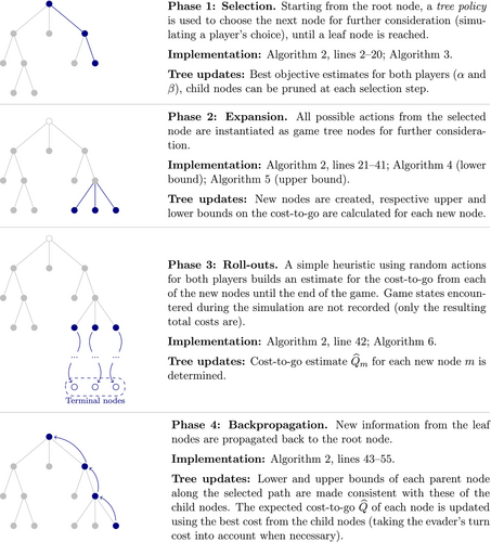
During Selection phase, a single strategy is sampled, which assumes a valid sequence of turns for both players. The key idea of the MCTS framework implies that each strategy is incorporated into the game tree only up to a certain (variable) depth, in terms of the number of players' turns, so that the strategies estimated to be closer to optimal will have higher depths. Further, we employ a classical pruning mechanism based on the upper and lower bounds presented in the literature. To balance exploration and exploitation of the action space, our reference implementation combines ideas from the multi-armed bandit literature and -greedy search.
The second phase, Expansion, increases the depth of the strategy chosen on the previous step. Child game tree nodes are created for all possible player actions in the state of last visited game tree node. Therefore, the selected strategy's depth is increased by one level. Note that while it is trivial to calculate the immediate payoff of each player action, such as the cost of traversing a single arc by the evader, the objective value accumulated until the end of the game remains unknown at this point.
The Roll-outs phase estimates these terminal values for the new game tree nodes. In particular, a series of random actions is assumed for both players until the game ends and the evader reaches the terminal point. Intermediate game states are not incorporated into the tree to save memory. Note that the closer the game tree node to the end of the game, the closer roll-out value would be to the true value of the strategy.
Finally, the Backpropagation phase performs a backward sweep, updating the values of being in the respective states of the game using the calculated bounds in the new leaf nodes and roll-out results along the chosen path in the game tree.
2.1 Implementation overview
Our algorithm builds a game tree whose nodes correspond to a partial game that has been played between the two players. The relevant information pertaining to the game is captured by state information, summarized in Table 1. We record state information pertaining to each node of the game tree. For a given node , the children of node in the game tree correspond to the new game state after an action is made at node .
| Notation | Description |
|---|---|
| Current evader's position; the game is concluded when . | |
| Interdiction decisions taken up to this point. | |
| The residual interdictor's budget, where . | |
| The player taking the next action at node . | |
| An estimate of the cost-to-go of the game starting from the state implied by node , assuming that player acts next. | |
| Lower and upper bounds on the cost-to-go of the game. | |
| Number of times the tree node was visited. | |
| List of child tree nodes, corresponding to the possible actions by player at game state implied by . | |
| Actions available to player that do not correspond to any existing child tree nodes. |
Our approach is a decision-time algorithm in the sense that it is designed to start from some current state of the game, represented by the root game tree node, and determine the next action to be taken by the corresponding player. After a decision is made, the child node corresponding to that decision becomes the new root node. All nodes not reachable from the new root node can be discarded, while information pertaining to nodes reachable from the new root node is retained.
Specifying all subsets of attacks for the interdictor can be computationally prohibitive. To avoid enumerating all possible attack subsets at each node corresponding to the interdictor's move, we impose the restriction that the interdictor can attack only one arc at each game tree node, while allowing the interdictor to retain its turn until the interdictor chooses to attack no further arcs (i.e., passes). We call these single-arc attack actions virtual turns for the interdictor. The evader's turn consists of a single arc to traverse; hence, there is no need to include virtual turns for the evader. We remove unnecessary symmetry from the interdictor's virtual turns by requiring that arcs can be attacked consecutively only in the increasing order of the tail node numbers. For example, arc must be attacked before within an uninterrupted sequence of single-arc attacks.
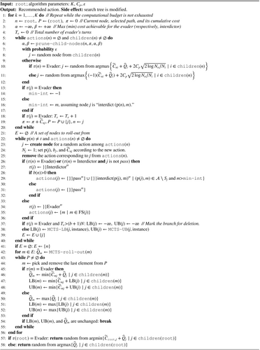
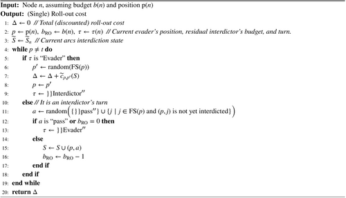
Algorithm 1 presents a high-level description of our approach. We initialize the game tree, evader position (), and game cost in the first two lines. Then, the algorithm repeatedly recommends the next action in line 4, leading to game tree node , until the evader reaches the terminal node. Line 5 updates the cost of the game, where cost is associated with an arc in the game tree. If game tree node corresponds to an interdictor's move, then ; else, is the cost of traversing arc . Hence, accumulates the total cost for the evader for the corresponding sequence of moves for both players. Lines 6 and 7 update the evader's position and the root node of the game tree, respectively.
The key function, MCTS-next-move, that finds the next action using MCTS appears in line 4 of Algorithm 1. We now give an overview of this critical function before describing the details.
Algorithm 2 provides pseudocode for MCTS-next-move. This function executes a sequence of MCTS iterations, which we call learning episodes, before deciding the next move to make. We break each learning episode into four stages, summarized in Figure 1. The Selection phase spans lines 2–20 of Algorithm 2. In this phase we start from the root node and recursively choose child nodes that are more promising according to our estimates, until we reach a leaf node of the game tree (not necessarily implying the end of the game). We also prune the tree as necessary during this stage. Then, during the Expansion phase (lines 21–41), we create child nodes for the selected node, corresponding to all possible actions that the current player can execute. We build an estimate for the future game cost (cost-to-go) for each new node during the Roll-outs phase by calling a procedure in line 42. In particular, starting from each new node we simulate a game by choosing player actions at random and record the resulting objective as the cost-to-go estimate, denoted . Finally, we propagate this new information back from the selected leaf node towards the root during the Backpropagation phase in lines 43–55. We traverse the tree backwards and update the cost-to-go estimates along with the bounds for each parent node to make them consistent with the information contained in the child nodes.
Finally, after learning episodes have been executed, the last two lines of the algorithm recommend an action depending on which player is acting at the root node. The evader will choose among the least-cost children of the root node, while the interdictor will choose from among the highest-cost children, given the arc traversal costs and the cost-to-go estimates established thus far.
The next four subsections provide algorithmic details for the four learning episode phases given above. Section 2.6 then discusses the correctness of our algorithm and its asymptotic convergence properties.
2.2 Selection
The result of the Selection phase is a path from the root node to a leaf node in the game tree. Node denotes the current game tree node in this path as we iterate from the root to a leaf node. We keep track of the selected nodes in ordered list (which initially contains only root), and the cumulative cost of the selected path in . The while-loop in line 5 iterates until node has no more children and no more unexplored actions that would generate more children. Given , the selection phase performs three tasks: pruning, node choice, and symmetry breaking.
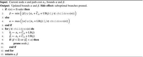
Pruning. We employ alpha–beta pruning [16] to mitigate the growth of the game tree. Recall that every game tree node is associated with a lower bound, , and an upper bound, , on the cost-to-go from node . These bounds are obtained in the expansion phase and are discussed in Section 2.3.
- : the worst (minimum) alternative cost achievable by the interdictor,
- : the worst (maximum) alternative cost achievable by the evader.
- For the evader's turn: ,
- For the interdictor's turn: .
The corresponding pseudocode is presented in Algorithm 3. After updating these and bounds, for every child node we calculate the lower bound and the upper bound on the total game cost assuming an optimal play starting from this child node. Then, we prune any child node of parent node such that or . Appendix A provides an illustration of alpha–beta pruning.
Node choice. One trade-off arising in our node choice task is one of exploration (exploring parts of the tree that have not yet been thoroughly examined) versus exploitation (searching areas of the tree that appear most promising). We employ the ideas of upper confidence bounds [17, 18] and -greedy search [38] to facilitate the exploration-exploitation trade-off.
An auxiliary variable takes the value of if “Interdictor,” and otherwise, and is used to accommodate the fact that the evader minimizes the game cost, while the interdictor maximizes it. Therefore, the first term represents our estimate for the additional game cost if we start from game tree node and proceed to node .
The second term is designed to make under-explored nodes more attractive. Note that as the total number of visits for the parent node increases, if children other than are selected more often, then will increase, making node relatively more attractive. The constant parameter regulates the degree of exploration and is chosen empirically. This term with the logarithm under the square root is inspired by research concerning the multi-armed bandit problem, as it captures the variance in the estimate of the action's value.
Multi-armed bandit research stems from the following problem. A user seeks to maximize expected profits in a sequential, repeated choice among discrete actions. Each action yields a (random) reward, but its distribution is unknown beforehand. Therefore, after several plays the user is faced with the exploration versus exploitation dilemma: one could either exploit actions for which much information is already known, or explore the action space in hope of finding one with a better expected reward, at a cost of experiencing actions with lower reward as well. A simple policy that achieves certain desirable theoretical properties for the -armed bandit problem, called UCB1, was proposed by [2].
In MCTS, despite its fully deterministic setting, the choice of a child node during our selection phase is a choice among a finite number of actions with uncertain rewards. (Uncertainty here arises from the lack of information regarding the consequences of the chosen strategy.) This analogy to the multi-armed bandit problem was exploited by [17, 18], who proposed an adaptation of UCB1 score to the MCTS setting (under the name Upper Confidence Bound for Trees, or UCT). A -armed bandit problem is discussed, for example, in [38, Section 2.1], and in the context of MCTS in [9, Sections 2.4 and 3.3].
Based on preliminary experiments, to speed up the procedure we also implement -greedy selection modification as follows. With probability we pick a child node uniformly at random. Otherwise (with probability ) we choose a node having the best score as described above. Note that this -greedy adjustment allows the algorithm to potentially consider any node within the game tree for exploration. We provide additional insights on selection strategies in Appendix C.
Symmetry breaking. Lines 13–17 ensure that no symmetric virtual turns are created for the interdictor. Here min-int tracks the to-node of the most recent arc that was interdicted, enforcing the anti-symmetry conditions stated previously for virtual turns. Lines 18 and 19 update the number of evader turns, costs, partial path, and current node.
2.3 Expansion
The expansion phase is described in lines 21–41 in Algorithm 2. We create child nodes of the current node corresponding to actions that can be taken from node . All such child nodes are placed in a list, .
To generate these child nodes, line 22 ensures that there are unexplored actions and that is not in fact the terminal node of the DSPI instance. Lines 23–25 create a new node , initializing the appropriate parameters and updating the unexplored actions from node . Lines 26–36 set up possible further actions for the new game tree node, ensuring that the tail node of an interdicted arc is always greater than that of the previous interdiction turn in an uninterrupted sequence of virtual attacks to avoid symmetry. Note that once we select a node, we create all possible child nodes at once.
Next, recall that our algorithm tracks the number of evader's turns in lines 4 and 18. We use this counter to limit the maximum tree depth in line 37. To justify this check, we establish the following lemma.
Lemma 1.For a DSPI instance given by a graph with nodes, initial interdiction budget , and nonnegative arc costs and interdiction increments, there exists an optimal solution involving no more than evader's turns.
Proof.Consider any optimal solution in which the evader takes more than than turns. Recall that there are positions for the evader on the DSPI graph, the interdictor's budget does not increase during the game, and the evader must change its position after every evader turn in the game. Define to be the interdictor's remaining budget at node of the game tree. Therefore, there must exist game tree nodes and corresponding to evader turns where and , where the turn at node precedes that at node . Because arc costs are nonnegative, and the evader's solution is assumed to be optimal, the evader must have accumulated zero cost in its traversals between game tree nodes and . Removing all such zero-cost cycle traversals, we obtain an alternative optimal solution that possesses the desired property.
Therefore, in our heuristic we discard any solution that implies more than evader's turns as follows. For the node corresponding to the first excessive evader's turn, we set upper bounds of all its child nodes to (line 37). By doing so, this node will be pruned during the next selection (involving this node) with any finite values of and .
Finally, assuming that a new node is not marked for deletion by Lemma 1, we establish lower and upper bounds on the cost-to-go from node . To do this, we adapt polynomial-time bounding strategies introduced in [32].
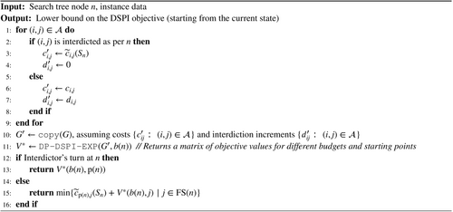
In particular, to obtain the lower bound, the interdictor is restricted by assuming that its attacks expire (i.e., are reset to their original, unattacked values) after the next evader's turn. Therefore, we need not keep track of the specific interdiction decisions , but just the residual budget. The corresponding polynomial-time algorithm in [32] is called DP-DSPI-EXP. Thus, our lower-bounding procedure, described in Algorithm 4, first incorporates the interdiction decisions already made from the path of the root node to node in the game tree, and then calls the dynamic programming algorithm DP-DSPI-EXP, which returns a matrix of the optimal objective values for each combination of the interdictor's remaining budget and evader's position.
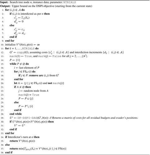
For the upper bound, we restrict the evader by removing arcs from the graph until it becomes a DAG. The removal of these arcs allows us to use the polynomial-time algorithm (which we denote DP-DSPI-DAG) given in [32] to solve the resulting auxiliary instance. The implementation is presented in Algorithm 5. We execute this algorithm NTRIALS=100 times (with each run removing possibly different arcs to form a DAG), and retain the best bound obtained.
2.4 Roll-outs
The prior expansion phase results in a list of newly created nodes having valid bounds, but with undefined cost-to-go estimates . To obtain cost-to-go estimates for the new nodes, the roll-out procedure is called in line 42 of Algorithm 2. The implementation described in Algorithm 6 plays out a game with uniformly random turns for both players. We track the game as it changes states in temporary variables that describe cost , the current evader's position , current budget , interdiction decisions , and turn .
2.5 Backpropagation
Note that given our approach to backpropagation, the algorithm is closely related to a minimax search [16], but uses the ideas of Monte Carlo simulations to estimate game costs and drive the search through the game tree.
2.6 Algorithm correctness and asymptotic properties
The MCTS algorithm we propose yields a valid sequence of turns and a heuristic objective estimate by construction. In this section we discuss some asymptotic properties pertaining to this algorithm. First, observe that the resulting game tree size is bounded in the following sense.
Lemma 2.The size of the game tree produced by Algorithm 2 (MCTS-next-move) is bounded by a finite function of the size of graph and the initial interdiction budget, .
Proof.First, suppose that is a DAG. For the evader, every turn implies traversing one of arcs, which is possible at most once in a DAG. Assuming all possible orders and no pruning, this yields at most distinct evader paths in the game tree. For every evader node, the interdictor can respond with possible actions, corresponding to different arc subsets in the forward star of a node in , where . Therefore, the total number of distinct sequences of moves captured in the game tree is at most . Because we never re-create game tree nodes corresponding to an already pruned game tree branch, the number of nodes is also bounded from above.
For a general graph, even in presence of nonnegative-cost cycles, similar logic applies. Lemma 1 allows us to limit the number of evader's turns we consider in each possible game to . Because every evader turn implies traversing an arc, there are at most options for each turn, so the total number of different evader's paths considered by our algorithm is no more than . Using the same logic as for the DAG case, the total number of turn sequences captured in the game tree is no more than before pruning. (Naturally, in our experiments, the tree is significantly smaller due to the pruning mechanism we discussed above. See also an illustration in Appendix B.)
In the foregoing proof, note in particular that the bound on the maximum size of the game tree depends only on , and is independent of the number of iterations, .
Theorem 1.Denoting the cost-to-go estimate at the root game tree node after learning episodes as and the true optimal objective as , the MCTS-next-move procedure implemented as per Algorithm 2 satisfies:
Proof.First, observe that if the algorithm recursively creates all the possible child nodes (which are finite in number as per Lemma 2), then there will be at least one path from the root to a leaf node in the game tree that would correspond to an optimal sequence of turns. Lemma 1 guarantees that if the algorithm expands all game tree nodes, then at least one root-to-leaf path remains optimal. Also, if all child nodes are instantiated in the game tree, then cost-to-go estimates for every node are exact cost-to-go values after a single pass of the back-propagation mechanism (2). Therefore, also equals the exact optimum, . Hence, the probability for is no less than the probability that the algorithm expands all possible game tree nodes. Because at each selection step we select a random node with probability , each possible node to expand will be selected with some positive probability bounded from below by some value . The probability that the algorithm will sample paths from the root node to all possible leaf nodes corresponding to the end of the game (given our pruning mechanism) is bounded from below by the probability of having the necessary (finite) number of successes, which we will denote , in a sequence of Bernoulli trials with success probability . As the target number of successful episodes does not depend on , the probability of having at least successes approaches 1 as grows indefinitely.
3 NUMERICAL EXPERIMENTS
To investigate the computational efficacy of the proposed algorithm, we performed a series of computational experiments over both pre-defined and randomly generated instances.
From [32], we used fifteen 10-node instances and fifteen 20-node instances of varying density, with the former having and the latter implying . Then, we generated a set of random instances using the Erdős-Rényi-Gilbert model [12] with varying number of nodes and parameter . That is, we created a completely connected graph, and then erased each arc with probability . Costs were generated as uniformly random integer numbers between 1 and 10, and interdiction were generated as uniformly random integer numbers between 0 and .
For all test instances, we ensured that every node was accessible from , and that was reachable from every other node in the graph. Nodes that did not possess these properties were deleted from the graph. Thus, a graph initially generated with nodes may contain fewer nodes after this preprocessing check, though few nodes were deleted in preprocessing.
Both the exact dynamic programming approach developed by Sefair and Smith and the MCTS algorithm proposed in this work were implemented from scratch using Julia programming language [7]. We ran all experiments on a laptop with a four-core Intel i5 processor (2.8 GHz) and 8 Gb of RAM. Unless stated otherwise, we chose parameter values , , and . These values were chosen after brief preliminary computational experiments. We note here that (affecting the exploration-exploitation trade-off) is problem-specific, and in principle could be normalized, for example, to the average pairwise shortest-path length in the graph.
3.1 Pre-defined instances and scaling
First, we run the MCTS algorithm against the dataset of pre-defined instances. Figure 2 depicts the known optimal value, calculated lower and upper bounds, and the objective obtained by our MCTS play-out for each instance. The bounds proposed by Sefair and Smith are very tight: in fact, they close the gap immediately for most instances. Although their bounds do not reveal the actual optimal policy, they direct our algorithm to find either optimal or near-optimal solutions in just learning episodes per move.
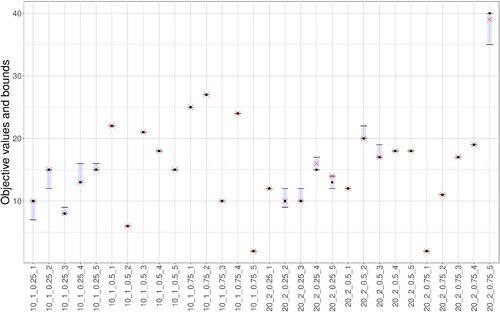
These instances were used to validate the exact approach, and are relatively easy to solve. The exact DP algorithm typically solved each instance in under 10 s (under 1 s most of the time), and was actually faster than our proposed heuristic on each instance. As one might expect, the exact and heuristic approaches scale in fundamentally different ways. To illustrate this fact, we modified each instance to consider the cases of , 2, and 3. We solved each of these new instances with the exact DP algorithm and using our MCTS procedure, keeping records of the runtime (in seconds) and the objective values obtained. The results are summarized in Table 2.
| Name | Runtime, sec. | Objective | ||||||||||||
|---|---|---|---|---|---|---|---|---|---|---|---|---|---|---|
| H | DP | H | DP | H | DP | H | DP | H | DP | H | DP | |||
| 10_1_0.25_1 | 10 | 61 | 0.13 | 0.00 | 0.65 | 0.08 | 1.00 | 3.68 | 10 | 10 | 10 | 10 | 10 | 10 |
| 10_1_0.25_2 | 10 | 61 | 0.20 | 0.00 | 0.24 | 0.08 | 0.71 | 3.21 | 15 | 15 | 19 | 19 | 19 | 19 |
| 10_1_0.25_3 | 10 | 61 | 0.27 | 0.00 | 0.55 | 0.08 | 0.89 | 3.60 | 8 | 8 | 10 | 10 | 11 | 11 |
| 10_1_0.25_4 | 10 | 61 | 0.28 | 0.00 | 0.59 | 0.08 | 0.72 | 3.81 | 13 | 13 | 17 | 17 | 22 | 22 |
| 10_1_0.25_5 | 10 | 61 | 0.24 | 0.00 | 0.44 | 0.10 | 1.06 | 3.79 | 15 | 15 | 19 | 19 | 19 | 20 |
| 10_1_0.5_1 | 10 | 41 | 0.26 | 0.00 | 0.39 | 0.03 | 0.52 | 0.81 | 22 | 22 | 24 | 24 | 24 | 24 |
| 10_1_0.5_2 | 10 | 41 | 0.08 | 0.00 | 0.09 | 0.02 | 0.37 | 0.89 | 6 | 6 | 8 | 8 | 8 | 8 |
| 10_1_0.5_3 | 10 | 41 | 0.14 | 0.00 | 0.18 | 0.06 | 0.29 | 0.97 | 21 | 21 | 28 | 28 | 31 | 31 |
| 10_1_0.5_4 | 10 | 41 | 0.07 | 0.00 | 0.21 | 0.02 | 0.19 | 1.06 | 18 | 18 | 24 | 24 | 28 | 28 |
| 10_1_0.5_5 | 10 | 41 | 0.33 | 0.00 | 0.20 | 0.03 | 0.26 | 0.99 | 15 | 15 | 15 | 15 | 15 | 15 |
| 10_1_0.75_1 | 9 | 16 | 0.11 | 0.00 | 0.14 | 0.00 | 0.20 | 0.03 | 25 | 25 | 26 | 26 | 35 | 35 |
| 10_1_0.75_2 | 9 | 20 | 0.09 | 0.00 | 0.09 | 0.00 | 0.17 | 0.07 | 27 | 27 | 40 | 40 | 44 | 44 |
| 10_1_0.75_3 | 2 | 1 | 0.00 | 0.00 | 0.00 | 0.00 | 0.00 | 0.00 | 10 | 10 | 10 | 10 | 10 | 10 |
| 10_1_0.75_4 | 8 | 16 | 0.05 | 0.00 | 0.10 | 0.00 | 0.16 | 0.03 | 24 | 24 | 26 | 26 | 26 | 26 |
| 10_1_0.75_5 | 9 | 20 | 0.06 | 0.00 | 0.16 | 0.02 | 0.31 | 0.07 | 2 | 2 | 2 | 2 | 2 | 2 |
| 20_2_0.25_1 | 20 | 271 | 1.30 | 0.02 | 1.77 | 3.03 | 5.22 | 1982.10 | 11 | 11 | 12 | 12 | 14 | 14 |
| 20_2_0.25_2 | 20 | 271 | 1.40 | 0.01 | 3.81 | 3.34 | 6.96 | 1845.37 | 8 | 8 | 10 | 10 | 10 | 12 |
| 20_2_0.25_3 | 20 | 271 | 0.62 | 0.00 | 3.94 | 2.62 | 9.38 | 1821.71 | 8 | 8 | 10 | 10 | 15 | 13 |
| 20_2_0.25_4 | 20 | 271 | 4.19 | 0.02 | 3.69 | 2.76 | 5.10 | 2539.39 | 13 | 13 | 16 | 15 | 16 | 18 |
| 20_2_0.25_5 | 20 | 270 | 8.83 | 0.01 | 3.35 | 2.82 | 6.53 | 1859.25 | 10 | 10 | 12 | 13 | 14 | 14 |
| 20_2_0.5_1 | 20 | 181 | 0.70 | 0.00 | 1.64 | 0.82 | 6.22 | 357.65 | 10 | 10 | 12 | 12 | 12 | 12 |
| 20_2_0.5_2 | 20 | 181 | 1.53 | 0.00 | 4.11 | 1.42 | 2.27 | 316.71 | 18 | 18 | 20 | 20 | 27 | 27 |
| 20_2_0.5_3 | 20 | 181 | 1.77 | 0.00 | 1.11 | 1.04 | 2.24 | 265.71 | 14 | 14 | 17 | 17 | 20 | 20 |
| 20_2_0.5_4 | 20 | 181 | 1.00 | 0.00 | 1.61 | 2.32 | 2.92 | 358.75 | 17 | 17 | 18 | 18 | 19 | 19 |
| 20_2_0.5_5 | 20 | 181 | 1.05 | 1.09 | 2.83 | 1.05 | 4.05 | 327.91 | 15 | 15 | 18 | 18 | 20 | 20 |
| 20_2_0.75_1 | 20 | 91 | 0.17 | 0.00 | 0.90 | 0.22 | 2.08 | 16.75 | 2 | 2 | 2 | 2 | 2 | 2 |
| 20_2_0.75_2 | 20 | 91 | 0.23 | 0.00 | 0.79 | 0.16 | 0.87 | 14.89 | 9 | 9 | 11 | 11 | 16 | 16 |
| 20_2_0.75_3 | 20 | 91 | 0.15 | 0.00 | 0.80 | 0.17 | 1.38 | 15.53 | 17 | 17 | 17 | 17 | 17 | 17 |
| 20_2_0.75_4 | 20 | 91 | 0.62 | 0.00 | 0.53 | 0.17 | 1.95 | 15.00 | 11 | 11 | 19 | 19 | 19 | 19 |
| 20_2_0.75_5 | 20 | 91 | 0.84 | 0.00 | 3.26 | 0.31 | 6.93 | 15.65 | 27 | 27 | 41 | 40 | 41 | 47 |
- Note: MCTS measurements are denoted as H (“heuristic”), and the exact algorithm is denoted as DP (“Dynamic Programming”). Discrepancies between the obtained objective values are highlighted with bold font. Instance names are provided in the format N_b_D_i as per [32], where N denotes the number of nodes before the preprocessing, b stands for the budget (in the original instance), D is the graph density characteristic, and i is an instance number.
First, note that for the majority of the cases the objective values coincide for both methods (except for a few larger instances). Therefore, 10 episodes per move was enough for the proposed algorithm to identify an optimal game play for both players in many cases on our dataset. This confirms our intuition that for larger instances, it would be prudent to allow larger computational budgets (increasing the value of ) to obtain better solutions.
Runtimes vary greatly but exhibit an expected pattern. When or 2, the MCTS was almost always significantly slower than the exact DP algorithm. However, even for the situation is reversed, as the state space of the DP grows exponentially, while the MCTS limits the game tree size via pruning and strategic move selection. Also as we would expect, these effects grow stronger as we move from the 10-node instances to the 20-node instances.
To further illustrate how the MCTS algorithm scales with the instance size, we generated three random fifty-node instances and varied the budget from to . The results are summarized in Figure 3. We still see that the MCTS approach often finds an actual sequence of turns leading to the optimal (or near-optimal) objective. The runtimes for these larger instances are under 100 s, which indicates that the MCTS-based approach is scalable for instances of this size, as opposed to the exact algorithm. The figure also suggests that for larger instances, we could trade off additional runtime for better solutions by increasing the maximum number of iterations , as the algorithm sometimes yielded play-out objectives outside of the calculated bounds. Note that obtaining objective values outside of the bounds is technically possible, because the algorithm chooses the actions based on our cost-to-go estimates. The bounds are not tight enough to cut off all suboptimal solutions. Also, note that the MCTS runtime does not grow as fast as increases from to as the exact DP algorithm would. The growth of the tree is evidently highly dependent on the instance structure.

3.2 MCTS convergence profile
Note that a naive implementation of our MCTS algorithm could ultimately construct a full minimax tree, which would inevitably find an optimal strategy given enough time and space. This section explores the ability of the MCTS heuristic to limit the exploration of the game tree while still obtaining high-quality solutions. To accomplish this analysis, we constructed a convergence profile of our heuristic as follows.
We generated a random instance having nodes, arcs, budget , arc costs between zero and , and an optimal objective between and (as determined by the procedures in [32]). We performed learning episodes from the same root node, varying between 0.05, 0.5, and 1.0. For each choice of , we executed Algorithm 2 from the original root node of the game tree, using learning episodes. We then recorded how four items changed as the algorithm iterated over each learning episode. These items are (a) the game tree size, (b) the iterations at which nodes are added to and pruned from the game tree, (c) the stability of the recommended action to take from the root node, and (d) the estimate of the game value. The results are summarized in Figure 4, where the four metrics are illustrated in each row, and the three columns correspond to the choice of . In particular, the “Added/pruned” charts show how many nodes were added (above the horizontal axis, in blue) or pruned (below the horizontal axis, in red) at each iteration. Also, for “Best action,” we arbitrarily index each possible action with a number and plot a dot corresponding to the action recommended at the current episode number (so that long horizontal lines indicate stability in the recommended action from the root node). Rows for the first and last metric are self-explanatory.
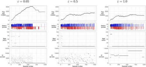
On the left panel, corresponding to , the tree grows very actively until around the 600th iteration. Pruning happens frequently as well, but at a slower rate than nodes are added. As the algorithm collects more information, the pruning starts to dominate and the game tree starts to shrink, until its size hits a plateau. In fact, we observe several plateaus interrupted by moments when valuable node discovery allows the algorithm to prune several game tree nodes. The tree size stops changing frequently after approximately 750 episodes, which is the point where the algorithm converges to a relatively stable cost estimate (at the root node) and a recommended action.
The nature of backpropagation with the minimum or maximum function makes the process unstable in terms of cost estimates: the cost-to-go at the root node varies from to about until around 600th episode. Recommended actions from the root node also change significantly, until they stabilize after around the 250th episode.
These four items vary significantly as we modify . For new node creation and pruning continue to occur regularly throughout all of the episodes, and while the game tree remains smaller on the average, the cost estimate at the root node struggles to converge to the optimum game value, only starting to achieve stability around episode 1000. Next, in the extreme case of a purely random exploration mode () the tree is kept even smaller, but our cost estimate never approaches its true value over the course of the first 1000 episodes. Therefore, deliberately excluding the mechanism of heuristic selection significantly deteriorated the performance of our algorithm.
We next verified that the difference in these convergence profiles is not simply due to the randomness employed in those algorithms. To do so, we performed three independent runs for each set of parameters, and observed the corresponding tree size dynamics as a function of the number of episodes. The results depicted in Figure 5 demonstrate that the algorithm behaves in roughly the same qualitative manner depending on the value of . That is, we see the same growth-and-pruning pattern when , and a more uniform growth pattern when or 1.0.
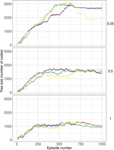
Note that when , our estimate stabilized around the optimum after more than 500 iterations. However, making turns and updating the root node itself seems to introduce another benefit of (heuristically) focusing the search process. We illustrate this effect in the following experiment.
3.3 The value of a play-out
Note that in the third row of panels in Figure 4, the next action recommendation stopped varying significantly earlier than the cost estimate, regardless of our choice of . Actually committing this move would have caused the algorithm to focus the analysis on a more promising alternative, ignoring the (now impossible) other moves. To investigate this effect, we generated random instances having 50 nodes each, with . We discarded any instance for which the initial optimality gap was positive, so that for all 250 instances, we know the optimal objective (but not an optimal sequence of moves). Each such instance was solved by the usual MCTS play-out algorithm, but this time we recorded the total number of learning episodes across all moves until the end of the game. After that, we re-solved the same instance starting from an empty game tree, allowing the algorithm to run for exactly the same number of episodes, but without making any moves. That is, in the latter case the algorithm started the selection every time from the initial root node. The results are summarized in Figure 6. The first row represents the full-tree approach, that is, trying to build an estimate for the best cost without making any moves. The bottom row represents the play-out strategy, when we run ten learning episodes followed by a turn repeatedly until the end of the game. The left column shows the histograms of the objective values obtained by the algorithms, relative to the true optimum. The right column presents the histograms of runtimes per instance, in seconds.
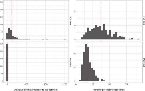
As one might expect, focusing the search by making a move after a limited number of learning episodes yielded improvements both in terms of objective value and runtime. (Mean runtimes, indicated by vertical dashed lines in the figure, differ by more than ten seconds per instance.) For our class of instances, we thus recommend updating the root node as a practical way to speed up the heuristic without significantly compromising solution quality.
4 CONCLUDING REMARKS
We focused on the DSPI problem, a complex variant of the shortest-path interdiction problem. A decision variant of the DSPI is known to be NP-hard, and an exact algorithm presented in the literature reduces to enumerating all the relevant states in a dynamic programming fashion. While existing research discusses bounds for the optimal game cost, our work contributes the first heuristic that provides solutions for the problem.
We have showed how several ideas from the game-playing and RL literature can be applied to this problem, and presented a heuristic algorithm based on the MCTS framework. Our approach creates a game tree that is used to recommend actions in turn for both players. In this manner, the approach “plays out” a DSPI instance. We demonstrate the practicality of the proposed approach over a series of numerical experiments and show that several key algorithmic components significantly contribute to the performance: guiding the search with cost estimates, pruning, and focusing the tree before making actual turns.
There are several possible future ideas that can be explored to improve the algorithm. One idea is to cache the most frequently used states of the game and share the information between the game tree nodes. Two such approaches discussed in the literature include “transposition tables” (when the most-visited game states share information across several nodes), and the idea of so-called “all-moves-as-first” roll-outs [9]. Another avenue for improvement might address the selection and roll-out processes. For the game of Go [34], neural networks were successfully used both for (randomized) node selection and roll-outs. It might be worthwhile to employ the idea of neural networks that are aware of the graph structure such as graph neural networks, see, for example, [1, 31, 41, 43]. It would be especially interesting to learn some patterns that would be persistent between different DSPI instances. Finally, we recommend future research that generalizes the MCTS approach here to solve other variations of dynamic interdiction problems.
APPENDIX A: PRUNING EXAMPLE
Consider a simple game tree presented in Figure A1. The interdictor's nodes are marked with “I,” and the evader's with “E.” We indicate the bounds on the cost-to-go for selected nodes in the figure. Assume that we have just expanded node on the left branch, node has an upper bound on the cost-to-go of , and the corresponding arc traversal yields cost . Further, assume that node has a lower bound of and an upper bound of . Then, an upper bound on the total game cost for node will be . We claim that node cannot be a part of an optimal solution, because it would be strictly better for the interdictor not to allow the evader to reach game state at all, by choosing node instead from the root node. This logic is implemented by our algorithm as follows. After the child nodes of were created and roll-out identified the cost-to-go estimates (which are irrelevant for the pruning mechanism), the backpropagation step will ensure that an upper bound for node is at most , due to formula (3). At the next learning episode, will be set to , due to the presence of node . An upper bound on the total game cost estimate for node will be . Because , node will be pruned during the selection phase, preventing it from being explored further.
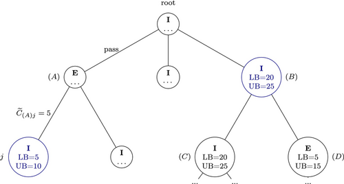
The pruning mechanism also works on the same level of nodes. Assume, for instance, that during the selection phase we have selected node . Choosing node would never be optimal for the interdictor, because the maximum path cost it can achieve there is 15, while node guarantees a cost of at least 20. In this case, , but after selecting node , the running lower bound will become at least . Therefore, the condition will trigger the pruning of node . Note that the symmetric pruning condition describes similar cases from the evader's perspective.
APPENDIX B: EXAMPLE ON THE INTERPLAY BETWEEN CYCLES AND PRUNING
In this appendix we will illustrate how the pruning mechanism limits the game tree size growth even in presence of a positive-cost cycle. Consider graph presented in Figure B1A. In the following, we denote nodes of as circled numbers, like ➀, to avoid confusion with the game tree nodes, which we will denote with capital Latin letters. A simple cycle is created by arcs ➀–➁ and ➁–➀, having costs and respectively. As before, we will restrict our attention to the evader's turns (as if the interdictor had no remaining budget.) In this case, the alpha–beta pruning mechanism will be dealing with the worst (maximum) alternative cost achievable by the evader (), and the minimum alternative cost achievable by the interdictor () will reduce to the best upper bound on alternative paths available to the evader.
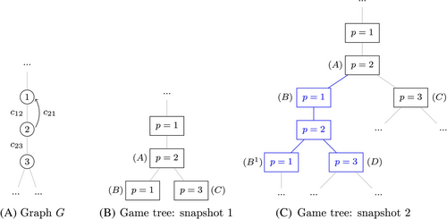
Consider a snapshot of a tree after expansion of the first game tree node corresponding to the evader's position at node ➁, depicted in Figure B1B. There are two child nodes, one of which corresponds to traversing the cycle and returning to node ➀. We show that expansion of this subtree according to the proposed algorithm will never yield unbounded growth of the game tree. First, if node is pruned, then the result follows trivially, so let us consider the case in which is not yet pruned. Expanding game tree node creates new game tree nodes describing the same possible actions from node ➀, as shown in Figure B1C. We show that such repeated blocks will be created only a finite number of times (with the bound not depending on ) due to the pruning mechanism. Let us denote the first “” node of the th additional block of nodes in a game tree (a copy of the nodes represented in Figure B1B) as . Note that a lower bound on the total game cost for node is , where comprises the total game cost up to node . However, during the selection phase, as we traverse the game tree from down to , the upper bound on the alternative path cost will be set to no more than . Therefore, there is a last redundant block comprising a subtree rooted at some node , which will be pruned no later than after new blocks will be created.
If the subtree with repeated actions grows beyond a certain limit (determined by the cost of the arcs creating the cycle) the algorithm will prune it in favor of alternative paths through the tree, for example, node against node in this example. Note that pruning does not eliminate all redundant nodes. For example, several repeated blocks might be created before we hit the pruning condition, and due to random roll-outs node could be deemed better than . So, a good solution might be found later in a subtree rooted at , but we would still have node in the game tree, representing exactly the same evader's position at ➂. Therefore, a zero-cost cycle might create a large, but finite multiplicative increase in the game tree size, with the bound not depending on the number of episodes .
APPENDIX C: ALTERNATIVE SELECTION STRATEGIES
Choice of an appropriate node selection scheme for an MCTS algorithm is an interesting research question. In Section 2.2, we employed a classical variant to show the performance of the basic MCTS algorithm applied to DSPI, with an additional -greedy selection step to improve solution quality. In this appendix we explore alternative selection strategies. See [9] and [39, Sections 2.2 and 3.2] for summaries of strategies that inspire our ideas here. Benchmarking different child node scores (for example, in terms of runtime or solution quality), as well as comparison of their theoretical properties in different settings, constitute a future research direction.
We first present a numerical illustration. We generated a single DSPI instance as discussed in Section 3, with 100 nodes, 2458 edges, edge costs distributed between 0 and 30, and the interdictor's budget of 3 arcs. The parameters were chosen so that the instance would be nontrivial to solve, with a positive gap between the lower (19.0) and upper (23.0) bounds.
We then performed three consecutive runs to construct a game tree after 1000 episodes for each of the following six alternative node selection strategies.
-greedy. With probability , we choose a child node at random. Otherwise, we pick one with the best value estimate, without the UCT term, that is, maximizing .
-UCB. Our reference implementation, described in Section 2.2. Namely, with probability we choose the child node uniformly at random, and one having the best UCB score otherwise.
We compared these three approaches to the following ad-hoc, heuristic alternative.
First, note that in all experiments the algorithm converged to a solution having the objective value between the upper and lower bounds. Therefore, the quality of the solutions were comparable.
Figure C1 summarizes the effect of the different strategies on the game tree. Each panel corresponds to a single selection strategy. We performed three runs per panel to illustrate the variation stemming from the randomness within the algorithm (and not the differences between the strategies). Episode numbers are along the horizontal axis, and the game tree size is along the vertical axis.
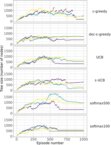
We see that -greedy strategy tends to keep the tree relatively large, exploring randomly chosen options consistently. The decaying -greedy strategy seems to benefit from active exploration in the beginning, and switches to the exploitation mode closer to the second half of the experiment, providing a relatively fast convergence. In fact, with carefully chosen decay parameters, the performance of this approach is comparable to our reference implementation of -UCB and UCB strategies. Note, however, that good parameter choices for and are not necessarily known in advance. Therefore, in practice this approach may require preliminary experimentation before it can be gainfully used. Finally, we were able to achieve competitive game tree dynamics with the softmax strategy. A higher temperature parameter yields more exploration in the first half of the experiment, even as compared to the -greedy strategy. This resulted in noticeably larger game trees. For the lower temperature value, the convergence was even faster than with the UCT variants. Note, however, that this heuristic approach does not necessarily allow for theoretical analysis, and may not retain the asymptotic properties enjoyed by other strategies.
The MCTS framework that we design for MCTS here allows for enough flexibility to accommodate many different improvements. For specific further ideas that can improve MCTS-based algorithm for DSPI we refer to the overviews in [9] and [39].
Open Research
DATA AVAILABILITY STATEMENT
The data that support the findings of this study are available from the corresponding author upon reasonable request.


