k-t GRAPPA accelerated four-dimensional flow MRI in the aorta: Effect on scan time, image quality, and quantification of flow and wall shear stress
Abstract
Purpose
The purpose of this study was to evaluate the utility of k-t parallel imaging for accelerating aortic four-dimensional (4D)-flow MRI. The aim was to systematically investigate the impact of different acceleration factors and number of coil elements on acquisition time, image quality and quantification of hemodynamic parameters.
Methods
k-t accelerated 4D-flow MRI (spatial/temporal resolution = 2.1 × 2.5 × 2.5 mm/40.0 ms) was acquired in 10 healthy volunteers with acceleration factors R = 3, 5, and 8 using 12- and 32-channel receiver coils. Results were compared with conventional parallel imaging (GRAPPA [generalized autocalibrating partial parallel acquisition], R = 2). Data analysis included radiological grading of three-dimensional blood flow visualization quality as well as quantification of blood flow, velocities and wall shear stress (WSS).
Results
k-t GRAPPA significantly reduced scan time by 28%, 54%, and 68%, for R = 3, 5, and 8, respectively, while maintaining image quality as demonstrated by overall similar image quality grading. Significant differences in peak WSS (diff12ch = −5.9%, diff32ch = 18.5%) and mean WSS (diff32ch = 13.9%) were found at the descending aorta for both receiver coils for R = 5 (PWSS < 0.04). Peak velocity differed for R=8 at the aortic root (−7.4%) and descending aorta (−12%) with PpeakVelo < 0.03.
Conclusion
k-t GRAPPA acceleration with a 12- or 32-channel receiver coil and an acceleration of 3 or 5 can compete with a standard GRAPPA R = 2 acceleration. Magn Reson Med 72:522–533, 2014. © 2013 Wiley Periodicals, Inc.
INTRODUCTION
Cardiac and respiratory gated three-dimensional (3D) CINE phase contrast (PC) MRI with three-directional velocity encoding (also termed “4D-flow MRI”) is an imaging technique enabling the measurement of 3D blood flow with full volumetric coverage of vessel systems such as the thoracic aorta. Several studies have demonstrated the utility of 4D-flow MRI for the 3D visualization and quantitative analysis of hemodynamic parameters such as flow velocities and wall shear stress (WSS) within the entire thoracic aorta 1-4.
Recent methodological advances including improved respiratory gating, parallel imaging, or fast sampling strategies such as radial imaging with 3D PC Vastly undersampled Isotropic PRojection (VIPR) allow aortic 4D-flow data acquisition in time periods on the order of 10–20 min 5, 6. However, total imaging time is still a limiting factor of this method and one of the reasons why it is often difficult to add 4D-flow MRI as a standard method in routine clinical practice.
Conventional parallel imaging such as SENSE (sensitivity encoding) 7 or GRAPPA (GeneRalized Autocalibrating Partially Parallel Acquisitions) 8 allow an acceleration R of PC data acquisition of up to R = 3 9; with the necessity to acquire some additional data in the k-space center (autocalibration lines for GRAPPA or training data for SENSE) the nominal acceleration Rnet is slower compared with R. The temporal domain has been used in TSENSE and TGRAPPA to omit these additional lines in central k-space yielding to Rnet = R 10, 11. More advanced spatio-temporal parallel imaging acceleration methods such as k-t SENSE 12 and k-t GRAPPA 13 or the recently introduced compartment-based k-t principal component analysis (k-t PCA) 14 have potential to further accelerate 4D-flow MRI. Previous reports have demonstrated the feasibility of such techniques to substantially reduce total 4D-flow scan time 15-17. However, it is known that k-t acceleration can induce temporal and spatial blurring and thus may impact 3D flow visualization and quantitative accuracy of the velocity data or derived parameters such as WSS.
To date, a 4D-flow MRI study analyzing the influence of different acceleration factors in k-t based parallel imaging and available coil elements used for signal reception on image quality and derived hemodynamic parameters is lacking.
In addition, none of the prior studies investigated the effect of spatio-temporal blurring of k-t acceleration on WSS evaluation or accuracy of WSS when compared with nonaccelerated 4D-flow MRI acquisition or with acceleration using standard parallel imaging such as SENSE or GRAPPA.
The aim of this study is to systematically investigate the performance of k-t accelerated 4D-flow MRI with respect to scan time reduction and potential loss of image quality and effect on quantification of flow velocities and WSS. A systematic analysis was performed using aortic 4D-Flow MRI in 10 healthy volunteers with the standard parallel imaging (PI) method GRAPPA and an acceleration factor of 2 (standard method) and k-t GRAPPA with acceleration factors 3, 5, and 8 and two different receive coils (12-channel and a 32-channel coil).
METHODS
Study Cohort
Ten healthy volunteers (6 males, 4 females, mean age 28.4 years ± 2.4, mean mid-ascending aortic diameters 27.4 mm ± 3.1 mm) were included in the study. The study was approved by the local institutional review board and informed consent was obtained from all participants.
MR Imaging
All measurements were performed on a clinical 3 Tesla (T) system (Trio, Siemens Medical Solutions, Erlangen, Germany) using a time-resolved 3D phase contrast gradient echo sequence with three-directional velocity encoding (velocity sensitivity along all directions = 150 cm/s). The 4D-flow data were acquired in a sagittal oblique 3D volume covering the entire thoracic aorta with TE/TR = 2.6/5.0 ms, flip angle = 7°, temporal resolution = 40.0 ms, spatial resolution = 2.1 × 2.5 × 2.5 mm3, bandwidth = 450 Hz/pixel. Data acquisition was synchronized with the cardiac cycle by prospective ECG gating and breathing artifacts were minimized by respiratory navigator gating as described previously by Markl et al 5.
For each volunteer, five 4D-flow MR acquisitions were performed during a single MRI examination. First, 4D-flow MR data were acquired using standard parallel imaging with undersampling along the phase encoding (ky) direction (generalized autocalibrating partially parallel acquisition, GRAPPA) with an acceleration factor of R = 2 using a 12-channel torso coil (Siemens Medical Solutions, Erlangen, Germany). Next, k-t accelerated 4D-flow MRI (i.e., undersampling along ky, kz, and t dimensions) with acceleration factors R = 3 and R = 5 was performed 15. Finally, the 12-channel coil was exchanged for a 32-channel torso coil (Siemens Medical Solutions, Erlangen, Germany) and 4D-flow MRI was executed with acceleration factors R = 5 and R = 8. The number of autocalibration (ACS) lines and the resulting nominal acceleration Rnet for the different acceleration factors R are summarized in Table 1. The total scan time for each acquisition was recorded.
| GRAPPA | k-t GRAPPA | ||||
|---|---|---|---|---|---|
| Coils | 12-channel | 12-channel | 32-channel | ||
| Acceleration factor R | 2 | 3 | 5 | 5 | 8 |
| ACS lines (Nky × Nkz) | Nky = 24 | 18 × 6 | 20 × 7 | 20 × 7 | 16 × 7 |
| Net acceleration Rnet | 1.6 | 2.8 | 4.2 | 4.2 | 6.3 |
| Nominal scan time | 25:36 | 14:34 | 9:30 | 9:30 | 6:06 |
| Scan time | 20:01 ± 3:13 | 14:30 ± 2:43 | 8:15 ± 1:33 | 10:14 ± 1:50 | 6:25 ± 1:03 |
- a Nky = autocalibration lines along phase encoding direction, Nkz = autocalibration lines along slices encoding direction, nominal scan time = total scan time based on 50% navigator efficiency and a heart rate of 60 beats / minutes, and the scan time averaged over all volunteers measurements.
Spatiotemporal Data Acquisition and Reconstruction
Spatiotemporal (k-t) undersampling of 4D-flow MR data and reconstruction was performed using the “PEAK GRAPPA” technique, an extension of k-t GRAPPA 13, as reported previously 18. Briefly, PEAK-GRAPPA is characterized by a uniform reconstruction kernel geometry composing a smallest cell within a ky-kz-t data undersampling pattern. Data sampling and reconstruction with different reduction factors (R = 3, 5, and 8) were performed as illustrated in Figure 1 using different sampling patterns and reconstruction kernels. In Figure 1 it is shown the source and target points used for calculating the coil weights and the reconstruction of the missing data. All partitions are acquired with the same pattern as shown in the ky-t plane for R = 3 and R = 5. Therefore, the reconstruction kernel comprises only one partition for these R factors. An interleaved acquisition pattern between adjacent partitions characterized by a shift of R/2 was acquired for R = 8. For R = 8, the reconstruction kernel comprises source points from three partitions. More details on the motivation or benefits of these sampling patterns and reconstruction kernels can be found in 15.
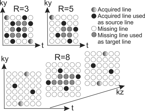
The k-t algorithm was integrated into the scanner's data reconstruction workflow and all undersampled data were acquired and reconstructed directly on the MR system.
Data Analysis-Preprocessing and 3D Blood Flow Visualization
The 4D-flow MRI data was preprocessed using in-house tools programmed in Matlab (The Mathworks, USA) to correct for aliasing, eddy currents, and background noise as described previously 19. A 3D PC MR angiogram (PC-MRA) was derived from the 4D-flow data by calculating the time averaged absolute velocity images weighted by the magnitude data for background suppression 19. Next, the preprocessed 4D-flow and 3D PC-MRA data were imported into commercial software (ENSIGHT 9.2, CEI, USA), which was used for 3D visualization of aortic blood flow and to position 2D analysis planes along the aorta. Intra-aortic blood flow was visualized using time-resolved pathlines originating from four emitter planes: aortic root, mid-ascending aorta, mid-aortic arch, and proximal descending aorta as illustrated in Figure 2.
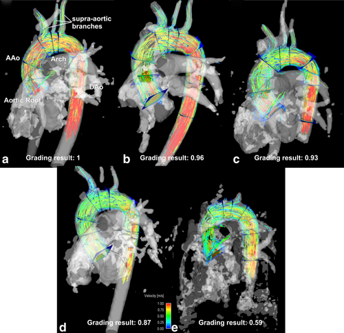
Image quality was semi-quantitatively evaluated by two independent, experienced observers who were presented with the PC-MRAs as well as a pathlines representation in a blinded, randomized manner. The visibility of the PC-MRA and the quality of the pathlines was graded based on separate Likert scales as noted below. PC-MRA quality grading was based on the depiction of the ascending aorta (AAo), the brachiocephalic trunk (bt), the left carotid artery (lCA), the left subclavian artery (lSA), and the descending artery (DAo) (all separately graded, 0 = not visible, 1 = partly visible, 2 = fully visible, see Fig. 2).
The 3D visualization quality was rated by visually examining the temporal evolution of pathlines over the cardiac cycle. Quality grading was based on the assumption that increased noise due to k-t undersampling would result in inaccuracies in particle trajectories and thus incomplete filling of the supra-aortic branches or the descending aorta (see Fig. 2). Incomplete filling was defined if pathlines did not reach further than the aortic arch and only into one of the supra-aortic branches. No filling was defined when pathlines only reached the ascending aorta and none of the supra-aortic branches. In specific, pathline visualization was evaluated on a 4-point Likert scale based on pathlines emitted from the aortic root (0 = no visible traces, 1 = pathlines reach only the AAo, 2 = pathlines reach aortic arch, 3 = pathlines reach the DAo). Visualization of flow to the supra-aortic branches was graded separately (0 = not visible, 1 = pathlines in only one branch, 2 = pathlines in two branches and 3 = pathlines in all 3 branches). All individual grading results were weighted by the maximum and are reported as a mean ± standard deviation of the two observers (best quality in each category = 1).
Data Analysis: Flow and WSS Quantification
For retrospective quantification of blood flow and WSS, four analysis planes were positioned at anatomic landmarks: plane 1 at the level of the aortic root, plane 2 in mid-ascending aorta at the level of the lower edge of the right pulmonary artery, plane 3 in the mid arch, and plane 4 in descending aorta at the same level as plane 2 (Figs. 2a and 3a). For each plane, the aortic lumen boundaries were manually segmented for each cardiac time frame using a home built tool programmed in Matlab (The Mathworks, USA). Flow quantification included the extraction of flow-time curves for each plane and the calculation of peak systolic velocity and net flow over the cardiac cycle.
The velocity gradient along the segmented vessel lumen contour was estimated using cubic spline interpolation as described previously to calculate WSS 20. The average WSS magnitude along the segmented vessel lumen contour was calculated for each plane and cardiac time frame. The mean absolute WSS (averaged over the cardiac cycle), and peak systolic WSS were determined.
Statistics
All continuous data are presented as means ± standard deviation. To compare the five different acceleration strategies with GRAPPA R = 2 with the 12-channel coil as standard method, a Lilliefors test was used to determine parameter normalcy. Once the distribution was classified a 1-way analysis of variance (ANOVA) (normal distribution) or the nonparametric Kruskal-Wallis (nonnormal distribution) test was performed to detect whether all samples are drawn from the same distribution. If a F or chi-squared statistic less than 0.05 determined that image quality, net flow, peak velocity, flow-time curves, or radiological grading results were significantly different between groups, a multiple comparisons test for all acceleration methods was performed 21. When the hypothesis of a Gaussian distribution was not rejected, independent-sample tests (two-sample t-test) were performed. Otherwise, the nonparametric Mann-Whitney U-test was used 22. The level of significance was adjusted for multiple testing (comparison of 5 methods) by Bonferroni correction (differences were considered significant for P < 0.05/5 = 0.01). To compare the flow time curves, the curves were averaged over all volunteers for each plane and truncated, so that the mean flow time curves for every tested method had the same length. All following steps were similar to the other tested parameters (as described above).
Different k-t acceleration methods were compared using Bland-Altman analysis analyzing mean differences (
 ) as well as limits of agreement (
 ± 1.96*dstd standard deviation of the differences).
The interobserver agreement at qualitative analysis was evaluated using Cohen's kappa 23.
RESULTS
For all 10 volunteers data were successfully acquired with the 12-channel coil for all planned acceleration factors. In three subjects, additional k-t accelerated GRAPPA with the 32-channel coil could not be performed due to an overall long scan session and limited subject compliance. As a result, a total of n = 30 12-channel (i.e., 10 for each of the scans GRAPPA R = 2, k-t GRAPPA R = 3, k-t GRAPPA, R = 5) and n = 14 32-channel (i.e., 7 for each of the scans k-t GRAPPA R = 5, and k-t GRAPPA, R = 8) 4D-flow data sets were available for analysis. A scan time reduction of 28% and 54% was achieved for k-t GRAPPA R = 3 and R = 5 (12-channel coil) and 54% and 68% for k-t GRAPPA R = 5 and R = 8 (32-channel coil), respectively compared with standard GRAPPA with R = 2 (Table 1).
3D Blood Flow Visualization
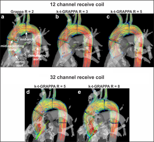
The 3D blood flow visualization for all five 4D-flow scans are shown in Figure 3. A similar distribution of pathlines and regional flow velocity magnitude (color coding) is appreciated across all acquisitions.
The results of qualitative 4D-flow image analysis are summarized in Table 2, demonstrating overall similar image quality for k-t accelerated 4D-flow MRI compared the standard acquisition (GRAPPA with R = 2). Increased acceleration factors results in a trend toward decreased quality scores which was, however, not significant (Kruskal-Wallis test for multiple comparisons). A higher number of coils for an acceleration factor of R = 5 (32-channel versus 12-channel) did not noticeably change image quality. Analysis of interobserver variability revealed almost perfect agreement (κ = 0.82).
| Category | 12-channel coil | 32-channel coil | |||
|---|---|---|---|---|---|
| GRAPPA R = 2 | k-t GRAPPA R = 3 | k-t GRAPPA R = 5 | k-t GRAPPA R = 5 | k-t GRAPPA R = 8 | |
| Visibility of PC-MRA, AAo | |||||
| mean ± std | 1 ± 0 | 1 ± 0 | 1 ± 0 | 1 ± 0 | 0.96 ± 0.09 |
| range | 1 – 1 | 1 – 1 | 1 – 1 | 1 – 1 | 0.5– 1 |
| Visibility of PC-MRA, bt | |||||
| mean ± std | 1 ± 0 | 1 ± 0 | 1 ± 0 | 0.86 ± 0.23 | 0.93 ± 0.17 |
| range | 1 – 1 | 1 – 1 | 1 – 1 | 0 – 1 | 0.5 – 1 |
| Visibility of PC-MRA, lCA | |||||
| mean ± std | 0.93 ± 0.23 | 0.93 ± 0.16 | 0.58 ± 0.35 | 0.79 ± 0.28 | 0.68 ± 0.37 |
| range | 0 – 1 | 0 – 1 | 0 – 1 | 0 – 1 | 0 – 1 |
| Visibility of PC-MRA, lSA | |||||
| mean ± std | 1 ± 0 | 1 ± 0 | 0.98 ± 0.08 | 0.86 ± 0.18 | 0.93 ± 0.17 |
| range | 1 – 1 | 1 – 1 | 0.5 – 1 | 0.5 – 1 | 0.5 – 1 |
| Visibility of PC-MRA, DAo | |||||
| mean ± std | 1 ± 0 | 1 ± 0 | 1 ± 0 | 0.86 ± 0.23 | 0.82 ± 0.22 |
| range | 1 – 1 | 1 – 1 | 1 – 1 | 0.5 – 1 | 0.5 – 1 |
| Quality of Pathlines, aortic filling | |||||
| mean ± std | 1 ± 0 | 1 ± 0 | 1 ± 0 | 1 ± 0 | 1 ± 0 |
| range | 1 – 1 | 1 – 1 | 1 – 1 | 1 – 1 | 1 – 1 |
| Quality of Pathlines, filling of supra-aortic branches | |||||
| mean ± std | 0.97 ± 0.07 | 0.97 ± 0.1 | 0.95 ± 0.08 | 0.98 ± 0.06 | 0.93 ± 0.09 |
| range | 0.67 – 1 | 0.67 – 1 | 0.67 – 1 | 0.67 – 1 | 0.67 – 1 |
| Average Grade | 0.98 | 0.98 | 0.93 | 0.90 | 0.89 |
| Std Grade | 0.09 | 0.08 | 0.20 | 0.20 | 0.22 |
- a The mean and standard deviation of the two observers is presented, as well as the range of the values. All grades are weighted by the maximum possible to get values between 0 and 1.
Flow Quantification
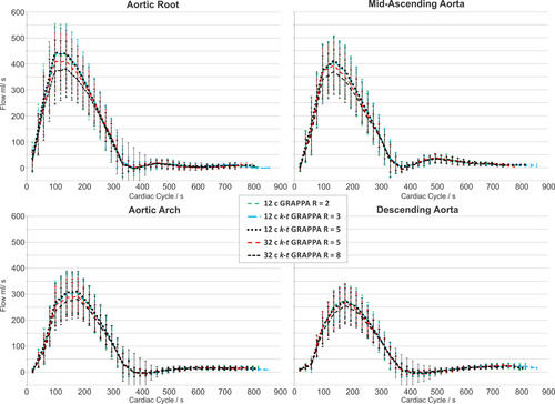
Figure 4 shows flow-time curves averaged over all subjects for different acceleration factors in all four analysis planes. Close agreement for all acceleration factors is clearly evident, which was confirmed by statistical analysis (Kruskal-Wallis test) showing no significant differences between flow-time curves distributions. At the aortic root, mid-AAo, mid-aortic arch, and proximal DAo 4D-flow MRI using the 12-channel and k-t GRAPPA with R = 3 led to only small differences in peak flow by 1.95%, 0.29%, 0.13%, and −2.24% compared with standard (GRAPPA R = 2). For the 12-channel and k-t GRAPPA with R = 5 differences were similar: 1.56%, 1.09%, 2.21%, and −1.67%. Measurements with the 32-channel coil and k-t GRAPPA with R = 5 underestimated peak flow by −5.31%, −3.69%, −4.19%, and −3.75%. 4D-flow MRI with R = 8 resulted in underestimation by −11.99%, −9.3%, −7.70%, and −7.95%.
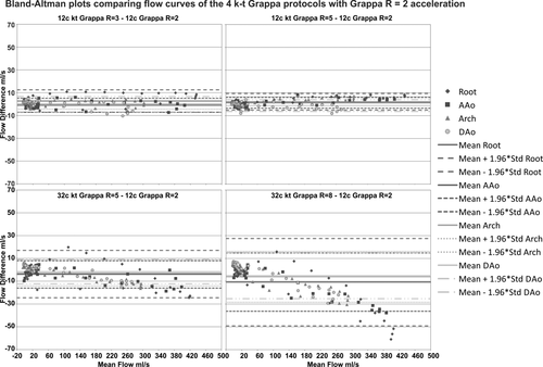
A detailed analysis of mean differences and limits of agreement are shown in the Bland-Altman plots in Figure 5 and in Table 4, revealing an increasing mean difference in flow curves for higher acceleration factors, with increased underestimation of peak flow.
Net Flow and Peak Velocity
Results for net flow and peak velocity quantification are summarized in Table 3. Net flow over the cardiac cycle was similar for all five methods and all planes (paired t-tests). Peak velocities were similar between methods except for the 32-channel k-t GRAPPA R = 8 configuration, which was significantly different from GRAPPA R = 2 at the aortic root and descending aorta (PPVelo_32R8,Root = 0.02, PPVelo,DAo = 0.03). The results of Bland-Altman comparisons (mean differences and limits of agreement) are summarized in Table 4. Similar to the flow time curves, net flow and peak velocity showed an increased mean difference for higher acceleration factors (Table 4).
| 12-channel coil | 32-channel coil | |||||||||
|---|---|---|---|---|---|---|---|---|---|---|
| GRAPPA R = 2 | k-t GRAPPA R = 3 | k-t GRAPPA R = 5 | k-t GRAPPA R = 5 | k-t GRAPPA R = 8 | ||||||
| Peak velocity (m/s) | Net flow (ml/cycle) | Peak velocity (m/s) | Net flow (ml/cycle) | Peak velocity (m/s) | Net flow (ml/cycle) | Peak velocity (m/s) | Net flow (ml/cycle) | Peak velocity (m/s) | Net flow (ml/cycle) | |
| Root | 1.30 ± 0.16 | 88.3 ± 26.3 | 1.28 ± 0.11 | 89.6 ± 22.6 | 1.26 ± 0.14 | 88.3 ± 20.4 | 1.30 ± 0.08 | 85.8 ± 22.0 | 1.21 ± 0.16a | 80.4 ± 21.4 |
| Mid-ascending aorta | 1.14 ± 0.19 | 86.1 ± 21.8 | 1.11 ± 0.16 | 86.3 ± 20.4 | 1.09 ± 0.18 | 86.8 ± 19.3 | 1.07 ± 0.16 | 84.2 ± 18.5 | 1.06 ± 0.20a | 79.4 ± 17.1 |
| Mid-arch | 1.05 ± 0.13 | 66.4 ± 18.1 | 1.03 ± 0.11 | 66.8 ± 17.5 | 1.03 ± 0.12 | 67.0 ± 17.5 | 1.03 ± 0.08 | 64.4 ± 15.1 | 0.99 ± 0.09 | 62.0 ± 14.0 |
| Descending aorta | 1.31 ± 0.16 | 59.7 ± 15.4 | 1.28 ± 0.15 | 60.2 ± 12.9 | 1.27 ± 0.21 | 58.6 ± 13.5 | 1.24 ± 0.09 | 59.0 ± 15.3 | 1.17 ± 0.12a | 56.1 ± 13.6 |
| Mean WSS (Pa) | Peak WSS (Pa) | Mean WSS (Pa) | Peak WSS (Pa) | Mean WSS (Pa) | Peak WSS (Pa) | Mean WSS (Pa) | Peak WSS (Pa) | Mean WSS (Pa) | Peak WSS (Pa) | |
| Root | 0.37 ± 0.06 | 1.07 | 0.36 ± 0.06 | 1.02 | 0.34 ± 0.07 | 0.95 | 0.33 ± 0.18 | 0.97 | 0.42 ± 0.11 | 1.12 |
| Mid-ascending aorta | 0.29 ± 0.04 | 0.73 | 0.29 ± 0.04 | 0.75 | 0.27 ± 0.04 | 0.67 | 0.29 ± 0.05 | 0.77 | 0.30 ± 0.04 | 0.79 |
| Mid-arch | 0.30 ± 0.05 | 0.78 | 0.29 ± 0.04 | 0.77 | 0.29 ± 0.05 | 0.76 | 0.33 ± 0.03 | 0.89 | 0.33 ± 0.04 | 0.81 |
| Mid-descending aorta | 0.36 ± 0.05 | 0.91 | 0.35 ± 0.05 | 0.87 | 0.35 ± 0.07 | 0.86a | 0.41 ± 0.04a | 1.08a | 0.40 ± 0.06 | 1.00 |
- a Significant difference in mean compared to GRAPPA R = 2 using paired t-test or Mann-Whitney U-test at P = 0.05 as significance level.
| 12-Channel k-t GRAPPA R = 3 | 12-Channel k-t GRAPPA R = 5 | 32-Channel k-t GRAPPA R = 5 | 32-Channel k-t GRAPPA R = 8 | |||||
|---|---|---|---|---|---|---|---|---|
Mean difference
 |
 ± 1.96 × SD ± 1.96 × SD |
Mean difference
 |
 ± 1.96 × SD ± 1.96 × SD |
Mean difference
 |
 ± 1.96 × SD ± 1.96 × SD |
Mean difference
 |
 ± 1.96 × SD ± 1.96 × SD |
|
| Peak velocity m/s | ||||||||
| Root | 0.02 | +0.22/ −0.17 | 0.04 | +0.26/−0.18 | 0.05 | +0.23/−0.13 | 0.14 | +1.36/−0.18 |
| AAo | 0.03 | +0.22 / −0.16 | 0.05 | +0.37/−0.27 | 0.12 | +0.45/−0.21 | 0.13 | +0.44/−0.19 |
| Arch | 0.01 | +0.20 / −0.17 | 0.02 | +0.18/−0.14 | 0.03 | +0.20/−0.15 | 0.07 | +0.26/−0.11 |
| DAo | 0.03 | +0.16 / −0.10 | 0.04 | +0.19/−0.12 | 0.07 | +0.28/−0.13 | 0.14 | +0.39/−0.11 |
| Net flow ml/cycle | ||||||||
| Root | −1.21 | +20.09/−22.51 | 0.25 | +20.92/−20.43 | −0.86 | +24.02/−25.74 | 4.38 | +23.18/−18.81 |
| AAo | −0.15 | +9.37/−9.67 | −0.68 | +10.61/−12.12 | −1.27 | +11.23/−13.77 | 3.62 | +22.06/−14.83 |
| Arch | −0.53 | +7.83/−8.90 | −0.82 | +5.52/−7.16 | −0.22 | +4.99/−5.43 | 2.18 | +13.74/−9.38 |
| DAo | −0.45 | +11.01/−11.92 | 1.17 | +9.58/−7.24 | −1.27 | +14.35/−16.89 | 1.39 | +13.96/−11.18 |
| WSS /Pa | ||||||||
| Root | 0.002 | +0.09/−0.002 | 0.03 | +0.14/−0.03 | 0.08 | +0.45/−0.08 | −0.01 | +0.19/+0.01 |
| AAo | 0.008 | +0.09/−0.008 | 0.02 | +0.08/−0.02 | 0.02 | +0.13/−0.02 | 0.01 | +0.11/−0.01 |
| Arch | 0.020 | +0.07/−0.02 | 0.02 | +0.09/−0.02 | 0.00 | +0.13/0.00 | −0.01 | +0.13/+0.01 |
| DAo | 0.020 | +0.09/−0.02 | 0.01 | +0.09/−0.02 | −0.03 | +0.05/+0.03 | −0.02 | +0.11/+0.02 |
| Flow curves ml/s | ||||||||
| Root | −2.69 | +7.10/−12.47 | −2.19 | +5.09/−9.48 | 3.75 | +24.54/−17.04 | 10.85 | +49.18/−27.47 |
| AAo | 1.08 | +7.22/−5.06 | −1.29 | +3.47/−6.06 | 4.05 | +16.05/−7.94 | 10.76 | +36.36/−14.84 |
| Arch | −0.15 | +4.52/−4.82 | −1.66 | +3.26/−6.57 | 2.82 | +14.06/−8.42 | 6.11 | +28.42/−16.20 |
| DAo | 0.14 | +6.86/−6.58 | 1.13 | +6.33/−4.08 | 2.59 | +16.15/−10.97 | 5.09 | +25.32/−15.14 |
WSS Quantification
Figure 6 and Table 3 summarize the results of the WSS analysis. Multiple comparison tests (Kruskal-Wallis and ANOVA) showed no significant differences in WSS-time curves (Fig. 6) between 4D-flow acquisitions for all planes. Differences for systolic peak WSS at the aortic root, mid-AAo, mid-aortic arch and proximal DAo for the 12-channel receiver coil and k-t GRAPPA with R = 3 compared with Grappa with R = 2 were: −4.6%, 2.1%, −1.4%, and −4.8%. For the 12-channel receiver coil and k-t GRAPPA with R = 5, differences were −11.0%, −8.3%, −1.8%, and −5.9%. Measurements with the 32-channel coil and k-t GRAPPA with R = 5 over- or underestimated peak WSS by −8.9%, 5.6%, 14.7%, and 18.5% and R = 8 resulted in overestimation by 4.5%, 8.0%, 4.5%, and 9.5%. Peak WSS for k-t GRAPPA R = 5 for the 12- and 32-channel configurations were significant different for the DAo (PPeakWSS_R5DAo = 0.01, PPeakWSS_32R5DAo = 0.016).
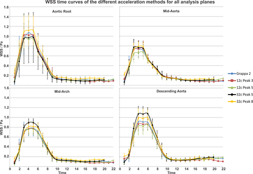
Mean absolute WSS showed no differences for acceleration factors R = 2, 3, and 5 in all planes for the 12-channel receiver coil configuration (Table 3). For the 32-channel receiver coil, the mean WSS in the DAo was significantly different for k-t GRAPPA R = 5 compared with GRAPPA R = 2 (PWSS_32R5,DAo = 0.04), whereas R = 8 did not differ significantly.
The results of Bland-Altman analysis for the WSS-time curves (summarized in Table 4) revealed moderate agreement for higher acceleration factors.
DISCUSSION
The results from this study demonstrate the feasibility of using advanced parallel imaging in combination with 4D-flow MRI for evaluating local and global aortic blood flow characteristics. The results revealed overall good image quality with low variability of the mean image grading, as indicated by the low standard deviations (SDs), and thus demonstrate the feasibility (i.e., improved scan efficiency) of using an advanced parallel imaging method such as k-t GRAPPA.
There were no significant differences between measured net flow, peak velocities and time-resolved flow curves at acceleration factor of 3 and 5 with the studied coil configurations. Mean peak velocity was significantly different from GRAPPA R = 2 at the aortic root and DAo for R = 8 (32-channel receiver coil). Net flow was less sensitive and revealed no significant differences. However, comparison of flow-time curves in Bland-Altman analysis showed high variability especially for the 32-channel receiver coil. The analysis of peak WSS was similar across all acquisitions except for the DAo for both receiver coils for the R = 5 acquisition. Mean WSS was significantly different from the standard GRAPPA method only for the k-t GRAPPA using the 32-channel receiver coil.
It should be noted that the analysis planes for the 12-channel and 32-channel coils were not identical as the data sets are not registered due to the change of coils during data acquisition. Nevertheless, care was taken that slice locations between the two coil setups were similar. The Bland-Altman comparison with standard GRAPPA R = 2 showed increased mean differences for both 32-channel coil measurements, the k-t GRAPPA R = 5 and R = 8. This was particularly evident for the flow time curves, which revealed an increasing underestimation of values with increasing flow values and acceleration factor. Analysis of peak velocities also showed increasing bias with increasing acceleration factor.
Based on our results for peak velocity and net flow, we conclude that the use of k-t accelerated 4D-flow MRI with high acceleration factors R = 5–8 is feasible. This results in a shortened measurement time of approximately 60% (12-channel k-t GRAPPA R = 5) when compared with the standard GRAPPA with R = 2.
However, quantitative blood flow analysis, which relies on the delineation of smaller features, including the identification of vessel and lumen boundaries for the calculation of WSS, k-t GRAPPA with acceleration factors larger than R = 3–5 may be problematic. Using a 12-channel coil with k-t GRAPPA of R = 3 reduced measurement time by 40% on average when compared with the standard GRAPPA with R = 2.
Noticeably, nonsignificant reduced peak velocities were observed for the 32-channel coil with k-t GRAPPA R = 5 in Figures 4 and 5, whereas the corresponding 12-channel results do not show this underestimation. A similar result has already been reported for two data sets acquired with a 12- and 32-channel coil, where the 32-channel coil did not show an improved estimation of peak velocities 15. It is assumed that the slightly inferior results of the 32-channel coil compared to the 12-channel coil are based on the lower sensitivity for more distant areas, such as the location of the aorta. For signals from tissue or blood flow closer to the surface coil elements, it is expected that the 32-channel coil will provide superior results.
Our standard method for comparison was GRAPPA reconstruction with an acceleration factor or R = 2. This method was thoroughly investigated in regards of reproducibility of flow and wall shear stress in a previous study 24. The authors tested reproducibility between observers and scans on 10 healthy subjects. Three planes were positioned along the aorta (ascending aorta, arch and descending aorta) by one observer. To test for interobserver variability, the vessel wall was manually segmented for all time frames by two independent observers. One of the observers repeated the segmentation to test for intraobserver variability. The scan-rescan variability was tested by repeating the scan on a second visit. Mean WSS and peak WSS showed significant agreement for reproducibly and good performance for inter- and intraobserver agreement. Mean differences for mean WSS stayed below 10% and for peak WSS below 9% (scan-rescan and observer differences). The comparison of the flow time curves between scans and observers showed good agreement and only small variations (scan-rescan and observer mean differences below 5%). Mean differences for peak velocity were below 3%.
Thunberg et al were the first to apply standard parallel imaging (SENSE) to 2D Cine PC-MRI revealing a robust and accurate estimation of peak velocities of up to R = 3 9. Several studies investigating PC-MRI with k-t acceleration methods followed based on standard parallel imaging with a reduction factor of R = 2 as reference. For example, Stadlbauer et al 25 investigated the performance of k-t BLAST acceleration (R = 2, 4, 6, 8) for hemodynamic parameter accuracy measured in the aorta with 2D Cine PC-MRI and compared the results with SENSE acceleration (R = 2) as well as ultrasound measurements. Results demonstrated that only an acceleration factor of R = 2 yields in no significant underestimation of peak velocities. Also, Baltes et al. 26 validated k-t SENSE and k-t BLAST (R = 5, 8) acceleration for the use in 2D phase-contrast MRI in the ascending aorta revealing a good agreement of flow parameters for R = 5 and a slight temporal low-pass filtering for an eight-fold acceleration.
To date, only a few studies investigated advanced acceleration techniques applied to 4D-flow MRI data, van Ooij et al 16 investigated phantom measurements of an intracranial aneurysm using k-t BLAST with R = 5 with and without SENSE (R = 3) acceleration. k-t BLAST resulted in a clear and SENSE in a moderate underestimation of peak velocities. The temporal blurring for both acceleration techniques decreased with increasing temporal resolution. Carlsson et al 17 showed that quantitative 4D-flow MRI accelerated with SENSE had good accuracy at 3T and 1.5T. Their experiments showed, however, that 4D-flow MRI accelerated with k-t BLAST with R = 5 clearly underestimated flow velocities and yielded too high bias for intracardiac quantitative in vivo use. They suggested SENSE or k-t BLAST for both field strengths for intracardiac 4D-flow MRI visualization. Another study by Stadlbauer et al 27 qualitatively and quantitatively compared time-resolved 3D MR velocity mapping from accelerated PC-MRI using k-t BLAST (R = 6) with PC-MRI using SENSE (R = 2) yielding a clear underestimation of peak velocities and also attenuations in blood flow dynamics with respect to streamline visualization, confirming the results of Carlson et al. Giese et al applied compartment-based k-t principal component analysis to 4D-flow MRI for the first time and retrospectively increased undersampling up to R = 8 without significant temporal blurring. Their results demonstrated much less temporal blurring than other k-t methods (such as k-t SENSE) resulting in an improvement of the accuracy of flow quantification 28. Hsiao et al investigated the effects of parallel imaging combined with CS on 4D-flow MRI derived parameters 29, 30, but only looked at interobserver agreement and 2D phase contrast MRI, without performing an analysis of hemodynamics or temporal blurring. The authors found overall good agreement between readers and good correlation between methods. All studies agreed that non-k-t acceleration produces more accurate results, but introduces more noise with faster acceleration than k-t acceleration, although k-t acceleration methods generally introduce temporal blurring.
A non-k-t acceleration method using radially undersampled acquisitions, the dual echo PC VIPR 6 was successfully applied in several 4D-flow PC-MRI studies 31, 32. In another study, the authors 33 could show that 4D PC VIPR provides reliable and reproducible measurements of pulse wave velocity, time-to-upstroke, time-to-peak, and time-to-foot measurements by comparison with 2D PC-MRI in the ascending and descending aorta.
Noticeably, previous results with an identical k-t GRAPPA reconstruction suggested feasibility of higher acceleration factors (R = 8) for 4D-flow measurements in the thoracic aorta using retrospectively undersampled data 15, which may give the impression that the acquisition of “true” undersampled data reduced the performance of the acceleration technique. However, in the previous study only two 4D-flow data sets with different coils have been investigated.
The quality of the reconstruction is not only influenced by the acceleration factor, but also the sampling pattern, the kernel configuration and the number of ACS lines. The kernel geometries within the sampling patterns were chosen to be less extended in partition direction as a more asymmetric data matrix with ky > kz is used in this study similar to many clinical applications. More details can be found in Jung et al 15. The number of the ACS lines was chosen according to the typical matrix size Ny × Nz as used for the aorta, i.e., with a similar ratio ACSy/ACSz ∼ Ny/Nz. For setting these values in the present study, the results obtained from the same previous study were used 15. No additional regularization has been used because an optimal selection of reconstruction kernels yields to a more pronounced enhancement of the reconstruction and further regularization does not improve results 34. Therefore, no additional tuning parameters (e.g., regularization or threshold parameters) were necessary for image reconstruction, as for instance in CS type reconstruction algorithms 35. On the other hand, it has been shown that CS improves the temporal fidelity of dynamic data compared with k-t BLAST reconstruction 36, which may result in higher acceleration factors when combining k-t GRAPPA and CS without enhancing low pass filter effects, as occurred in the flow curves for higher acceleration factors in our study.
Study Limitations
In this feasibility study, we only measured and analyzed a small study cohort, though the majority of participants had five data sets to analyze and manually segment. However, the impact of k-t acceleration on the assessment of disturbed blood flow in patients has not been investigated yet. In addition, we did not perform a direct comparison to imaging acceleration techniques other than GRAPPA and k-t GRAPPA. Also, we performed visual grading of image quality without quantitative analysis (SNR, g-factor, or root mean square error analysis) due to the spatial variation of image noise as a result of the parallel imaging reconstruction. The accurate estimation of regional noise would have required the acquisition of additional “noise only” data (by setting the flip angle to zero) which could not be performed in the framework of our already lengthy imaging protocols (five 4D-flow scans and coil change).
However, because 4D-flow MRI is still a relatively new method it is very important to think of quantitative measures to assess image quality. To date, there is no standardized procedure. We chose a semiquantitative image quality assessment of pathlines with defined grading categories. To be more objective, we asked two trained radiologists to grade the image and pathline quality using the defined criteria and we evaluated the interobserver agreement. Our well-defined grading system and the low interobserver variability (κ = 0.82) justifies this approach.
A limitation to the clinical applicability of k-t GRAPPA accelerated techniques is the reconstruction time. The reconstruction times for the 12- and 32-channel coil acquisitions averaged 5–10 and 30–60 min, respectively. The k-t GRAPPA based reconstruction process could be accelerated by a parallelization using GPUs, although this was not explored in our study.
It should be noted that our study focused on flow measurements in the thoracic aorta. However, the performance may vary with applications in other vascular territories, due to different volume locations and requisite differences in coil configuration.
We conclude that k-t GRAPPA acceleration with a 12-channel coil setup and an acceleration of R = 3 and R = 5 generates data of comparable visual quality with a standard GRAPPA R = 2 acceleration. A change of the number of channels of the coil from 12 to 32 did not significantly improve the results. The effects of higher acceleration factors have to be considered for the use in phase-contrast flow measurements. Further studies using other k-t acceleration methods and parallel imaging combined with CS are warranted, with the ultimate goal to define a technique with acceptable performance characteristics that enables application in the clinical setting.


