Understanding chicken walks on n × n grid: Hamiltonian paths, discrete dynamics, and rectifiable paths
Abstract
Understanding animal movements and modeling the routes they travel can be essential in studies of pathogen transmission dynamics. Pathogen biology is also of crucial importance, defining the manner in which infectious agents are transmitted. In this article, we investigate animal movement with relevance to pathogen transmission by physical rather than airborne contact, using the domestic chicken and its protozoan parasite Eimeria as an example. We have obtained a configuration for the maximum possible distance that a chicken can walk through straight and nonoverlapping paths (defined in this paper) on square grid graphs. We have obtained preliminary results for such walks which can be practically adopted and tested as a foundation to improve understanding of nonairborne pathogen transmission. Linking individual nonoverlapping walks within a grid-delineated area can be used to support modeling of the frequently repetitive, overlapping walks characteristic of the domestic chicken, providing a framework to model fecal deposition and subsequent parasite dissemination by fecal/host contact. We also pose an open problem on multiple walks on finite grid graphs. These results grew from biological insights and have potential applications. © 2014 The Authors. Mathematical Methods in the Applied Sciences published by John Wiley & Sons Ltd.
1 Straight walk and nonoverlapping walk
Parasitic pathogens with direct single-host life cycles rarely rely on aerial transmission for dissemination, more commonly featuring direct (i.e., physical contact) or indirect (environmental, food-borne or water-borne) routes 1. Examples include protozoans such as Cryptosporidium and Eimeria, helminths such as Ostertagia ostertagi and arthropods such as Sarcoptes scabei. Understanding the transmission of such pathogens requires an awareness of host movement as the initial source of pathogen spread, informed by subsequent environmental factors such as food movement, flow of water and other fomites. Recognition of the relevance of poultry to food security has elevated the importance of their pathogens, with parasites such as Eimeria of key significance 2. Eimeria can cause the disease coccidiosis, a severe enteritis characterized by high morbidity and, sometimes, mortality. The global cost of losses attributed to Eimeria and their control has been estimated to exceed $3 billion per annum, complicated further by welfare implications 3. Most Eimeria are absolutely host-specific and exhibit a strict fecal–oral life cycle including an environmental stage, called the oocyst, which must undergo a process termed sporulation over 12 to 30h external to the host in order to become infective. Thus, the physical behavior of chickens including the amount of time spent moving, the distance moved, the pattern of movement and the frequency and location of defecation while moving are of critical importance to understanding Eimeria transmission. Transmission rates have previously been calculated for Eimeriaacervulina 4. Overlaying these data onto models of chicken movement will support prediction of Eimeria transmission through a flock, facilitating scrutiny of the impact of management system and the opportunity for coinfection by genetically diverse parasite strains 5-7. The frequency of coinfection with genetically diverse strains will determine the rate at which cross fertilization may occur, influencing the occurrence of novel genotypes with relevance to evasion from drug-mediated and vaccine-mediated parasite killing 8. Inspired by the importance of chicken movement in Eimeria transmission, this work grew into an exercise to model chicken movement while studying the length of distance chickens walk per unit time in a pen, their parasite-disseminating characteristics and the rate at which infection spreads between birds. In order to understand the complexity of chicken movement, we have begun by assuming a square pen which can be subdivided into a cellular graph. The walks considered in this manuscript are of maximum length. By joining several such walks together in the future, we will begin to recreate multiple chicken paths as an entrée to modeling chicken movements in more complex environments.
Let us consider an area, S, of dimension n × n (n > 1) which is divided into n × n small squares (or cells). Let (i,j) be the cell which is located at ith row and jth column of these n cells. Suppose we leave a chicken in one of the cells of S and suppose we are interested in observing the walking behavior of the chicken through the following two rules: (i) walking from one corner point to a neighboring corner point and (ii) walking only through each cell (excluding on the cell boundaries). The (i,j)th cell is denoted by Sij[Ai,Bj,Cj,Di], where Ai, Bj, Cj and Di are four vertices of this cell that are located at the upper left corner, upper right corner, lower right corner and lower left corner, respectively. A chicken sitting inside the cell (i,j) (not on the vertices) is denoted by K(i,j), and a chicken sitting on the vertices Ai, Bj, Cj and Di of Sij is denoted by K(Ai), K(Bj), K(Cj) and K(Di) of Sij, respectively. A straight walk by K(i,j) is defined here as a walk initiated by K(i,j) for all i = 1,2,⋯,n and j = 1,2,⋯,n by moving to a neighboring cell through adjacent sides only, and a straight walk by K(Ai), K(Bj), K(Cj) or K(Di) of Sij, respectively, for all i = 1,2,⋯,n and j = 1,2,⋯,n is defined here as a walk from one cell to another cell that shares an edge with the current cell. For example, K(1,3) means that the chicken is in the cell which is at first row and third column and K(A2) of S23 means that the chicken is at the vertex A2 of cell S23 (which is located at second row and third column) which has four vertices [A2,B3,C3,D2].
We can visualize the area S either with even number of cells (2n × 2n) or with odd number of cells ((2n + 1) × (2n + 1)) and is placed on a grid graph, G, which is a subset of an infinite graph, G∞ 9. See 9-13 for foundations on grid graphs and 14-19 for infinite graphs. If an area S has (2n × 2n) cells, then it will have ((2n + 1) × (2n + 1))vertices. This gives us some flexibility to construct walks connecting some finite number of cells and relate such walks to the walks through vertices. Using the same flexibility, we define a cell as even if both i and j are even or i + j ≅ 0(mod2). Hence, a maximum possible walk between two cells (i,j) and (i*,j*) can be considered as a Hamiltonian path between these two cells. The problem of determining if a given graph G has a Hamiltonian path is NP-complete 9. We have described Hamiltonian and related paths through cells in a grid in section 2. The maximum paths between cells that we considered as described previously and further discussed in sections 3 and 4 are simpler situations than NP-complete problems. Our results indicate that maximum possible walks can be configured based on the position of the cells connecting walks in an even dimensional area and an odd dimensional area. Primarily, we differ in our approach because we tried all our attempts by connecting maximum possible walks between two cells. However, one can attempt to relate particular cases of our types of walks with Hamiltonian path configurations.
2 Related works
Our results were not inspired by previous work on Hamiltonian paths or NP-complete problems. We obtained the solutions of maximum possible walks from fundamental principles while trying to model chicken walks to understand transmission rates and cross fertilization of certain parasites with strict fecal/oral life cycles among chickens. We have thought of distributing the locations of defecations per unit of time, and hence we tried to link two Hamiltonian paths at these locations. Moreover, Hamiltonian path problems are related to the paths connected between two vertices. See 20, 21 for basic introduction to the Hamiltonian paths. Let G be a finite and simple graph with at least three vertices. Then, by Ore's Theorem 22, G is Hamiltonian if for every pair of nonadjacent vertices (say, a and b) the sum of the degrees of a and b is at least 3. Ore's Theorem is based on the arguments of the work by Newman 23, who proved that “Any graph with 2n vertices each of order not less than n must contain a 2n-gon.” A graph G is called Ore-type (k) if it satisfies d(a) + d(b)≥|G|+k, where d(a) and d(b) are degrees of a and b, respectively. G is k-path Hamiltonian if G is a graph on p vertices and d(a) + d(b)≥p + k for every pair {a,b} 24. In general, when G has p vertices, then G is k-path Hamiltonian if G has at least
 edges 24. This condition is sufficient for a graph to be k-path Hamiltonian. For works on the longest paths in undirected graphs (random), refer to 25-27. Algorithms for approximating the longest paths in grid graphs and meshes can be seen here 28-32. There are methods that are based on the longest paths in random graphs (for example, see 25) and search for the trees formed by probability processes 33, 34. Using the Turing machine-based models, computational complexity of k-path problems were studied (see 35), and for the importance of finding a path in a plane, see 36.
3 Maximum possible walk
In this section, we study the properties of obtaining maximum possible walks under the hypotheses of straight and nonoverlapping walks.
Theorem 3.1.(A) Suppose a straight walk is initiated by K(i,j) in S (the maximum distance covered by K(i,j) without stepping onto the same cell cannot exceed n2−1), then there exists configurations when the walk is initiated through any neighboring side of the K(i,j).
(B) Suppose a straight walk is initiated by K(Ai), K(Bj), K(Cj) or K(Di) of Sij in S (the maximum distance covered by each of these walks cannot exceed (n + 1)2−1), then there exists configurations when the walk is initiated through any neighboring vertex.
Proof.That the maximum distance traveled is n2−1 is easy to verify, so we will concentrate here on configurations. (A) We introduce notations for the directions of movement of a chicken between cells either rowwise or columnwise. A chicken moved from (i,j) to (i − 1,j) is denoted by the direction (i − 1)jdij; similarly, a move from (i,j) to (i,j + 1) is denoted by the direction i(j + 1)dij, a move from (i,j) to (i + 1,j) is denoted by the direction (i + 1)jdij and a move from (i,j) to (i,j − 1) is denoted by the direction i(j − 1)dij.
We prove the theorem in two situations, (I) when S has dimension 2n × 2n and (II) when S has dimension (2n + 1) × (2n + 1).
(I) S has dimension 2n × 2n.Consider a chicken in an arbitrary cell, (i′,j′), i.e., K(i′,j′). Suppose (2n − i′) is an odd number and (2n − j′) is an even number. This means that there are an odd number of columns to the right of K(i′,j′), an even number of columns to the left of K(i′,j′), an odd number of rows above K(i′,j′) and an even number of rows below K(i′,j′). We prove the statement for each of the four directions.
(a) The starting direction from K(i′,j′) is
 . Follow the configuration given in the steps shown subsequently:
(a1) Take (i′−1) steps in the direction
 to reach the first row; (a2) take (2n − i′) steps in the direction
 to reach the last column; (a3) take (2n − 1) steps in the direction 2(2n)d1(2n) to reach the last row; (a4) take one step in the direction (2n)(2n − 1)d(2n)(2n); (a5) take (2n − 2) steps in the direction (2n − 1)(2n − 1)d(2n)(2n − 1); (a6) take one step in the direction 2(2n − 2)d2(2n − 1); (a7) take (2n − 2) steps in the direction (2n)(2n − 2)d2(2n − 2) to reach the last row; (a8) repeat the steps similar to the steps (a4) to (a6) to reach the last row and (2n − j′+1) column where the given chicken is currently located, i.e., K(2n,(2n − j′+1)); (a9) take (2n − j′) steps in the direction
 to reach the first column; (a10) take (2n − 1) steps in the direction (2n − 1)1d(2n)1 to reach the first row; (a11) take one step in the direction 12d11; (a12) take (2n − 2) steps in the direction 22d12; (a13) take one step in the direction (2n − 1)3d(2n − 1)2; (a14) take (2n − 2) steps in the direction (2n − 2)3d(2n − 1)3 to reach the first row; (a15) take one step in the direction 14d13; (a16) take (2n − 1) steps in the direction 24d14; (a17) repeat the steps similar to the steps (a8) to (a16) such that the chicken is located in the (2n − 1) row and (2n − j′−1) column, i.e., K((2n − 1),(2n − j′−1)); (a18) take one step in the direction
 ; and (a19) take (i′−2) steps in the direction
 to reach the cell ((2n − i′+1),(2n − j′) such that we will have K((2n − i′+1),(2n − j′). This way the chicken takes 4n2−1 steps, and we achieved maximum distance configuration.
(b) The starting direction from K(i′,j′) is
 . The maximum distance configuration is given in the steps shown subsequently:
(b1) Take (2n − j′) steps in the direction
 to reach the last column; (b2) take (2n − i′) steps in the direction
 to reach the last row; (b3) take (2n − 1) steps in the direction (2n)(2n − 1)d(2n)(2n) to reach the first column; (b4) take one step in the direction (2n − 1)1d(2n)1; (b5) take (2n − 2) steps in the direction (2n − 1)2d(2n − 1)1; (b6) take one step in the direction (2n − 2)(2n − 1)d(2n − 1)(2n − 1); (b7) take (2n − 2) steps in the direction (2n − 2)(2n − 2)d(2n − 2)(2n − 1) to reach the first column; (b8) take one step in the direction (2n − 3)1d(2n − 2)1; (b9) take (2n − 2) steps in the direction (2n − 3)2d(2n − 3)1; (b10) repeat the steps similar to the steps (b6) to (b9) such that the chicken is located in the cell ((2n − i′+3),(2n − 1)), i.e., K((2n − i′+3),(2n − 1)); (b11) take two steps in the direction
 ; (b12) take one step in the direction
 ; (b13) take one step in the direction
 ; (b14) take one step in the direction
 ; (b15) take one step in the direction
 ; (b16) repeat the steps similar to the steps (b7) to (b15) to reach the cell ((2n − i′+1),1); (b17) continue for i′ steps in the same direction to reach the cell (1,1); (b18) take (2n − 1) steps in the direction 12d11 to reach the last column; (b19) take one step in the direction 2(2n)d1(2n); (b20) take (2n − 2) steps in the direction 22d2(2n); (b21) take one step in the direction 32d22; (b22) take (2n − 2) steps in the direction 33d32 to reach the last column; (b23) repeat the steps similar to the steps (b19) to (b22) such that the chicken is located in the cell ((i′−3),2n); (b24) take two steps in the direction
 ; (b25) take one step in the direction
 ; (b26) take one step in the direction
 ; (b27) take one step in the direction
 ; (b28) take one step in the direction
 ; (b29) repeat the steps similar to the steps (b25) to (b28) to reach the cell ((i′−1),2), i.e., K((i′−1),2); (b30) take one step in the direction
 ; and (b31) take (j′−1) steps in the direction
 to reach the maximum distance configuration.
(c) The starting direction from K(i′,j′) is
 . The maximum distance configuration is given in the steps shown subsequently:
(c1) Take (2n − i′) steps in the direction
 to reach the last row; (c2) take (j′−1) steps in the direction
 to reach the first column; (c3) take one step in the direction (2n − 1)1d(2n)1; (c4) take (2n − 2) steps in the direction (2n − 2)1d(2n − 1)1 to reach the first row; (c5) take one step in the direction 12d11; (c6) take (2n − 2) steps in the direction 22d12; (c7) repeat the steps similar to the steps (c4) to (c6) until the chicken is located in the cell ((2n − 1),(j′−3)), i.e., K((2n − 1),(j′−3)); (c8) take two steps in the direction
 ; (c9) take one step in the direction
 ; (c10) take one step in the direction
 ; (c11) take one step in the direction
 ; (c12) take one step in the direction
 ; (c13) repeat the steps similar to the steps (c10) to (c12) to reach the cell (1,(j′−1)), i.e., K(1,(j′−1)); (c14) take (2n − j′+1) steps in the direction
 to reach the last column; (c15) take (2n − 1) steps in the direction 2(2n)d1(2n) to reach the last row; (c16) take one step in the direction (2n)(2n − 1)d(2n)(2n); (c17) take (2n − 2) steps in the direction (2n − 1)(2n − 1)d(2n)(2n − 1); (c18) take one step in the direction 2(2n − 2)d2(2n − 1); (c19) take (2n − 2) steps in the direction 3(2n − 2)d2(2n − 2); (c20) repeat the steps similar to the steps (c16) to (c19) such that the chicken is located in the cell ((2n),(j′+3)), i.e., K((2n),(j′+3)); (c21) take one step in the direction
 ; (c22) take one step in the direction
 ; (c23) take one step in the direction
 ; (c24) take one step in the direction
 ; (c25) take one step in the direction
 ; (c26) repeat the steps similar to the steps (c22) to (c25) such that the chicken is located in the cell (2,(j′+2)), i.e., K(2,(j′+2)); (c27) take two steps in the direction
 ; (c28) take (i′+3) steps in the direction
 such that the chicken reaches maximum distance under the hypotheses.
(d) The starting direction from K(i′,j′) is
 . The maximum distance configuration is given in the steps shown subsequently:
(d1) Take (j′−1) steps in the direction
 to reach the first column; (d2) take (i′−1) steps in the direction
 to reach the first row; (d3) take (2n − 1) steps in the direction 12d11 to reach the last column; (d4) take one step in the direction 2(2n)d1(2n); (d5) take (2n − 2) steps in the direction 2(2n − 1)d2(2n); (d6) take one step in the direction 32d22; (d7) take (2n − 2) steps in the direction 33d32 to reach the last column; (d8) repeat the steps similar to the steps (d4) to (d7) such that the chicken is located at ((i′−1),2n), i.e., K((i′−1),2n); (d9) take (2n − i′+1) steps in the direction
 to reach the last row; (d10) take one step in the direction (2n)(2n − 1)d(2n)(2n); (d11) take (2n − 2) steps in the direction (2n)(2n − 2)d(2n)(2n − 1) to reach the first column; (d12) take one step in the direction (2n − 1)1d(2n)1; (d13) take (2n − 2) steps in the direction (2n − 1)2d(2n − 1)1; (d14) take one step in the direction (2n − 2)(2n − 1)d(2n − 1)(2n − 1); (d15) repeat the steps similar to the steps (d11) to (d14) such that the chicken is located at (i′,(2n − 1)), i.e., K(i′,(2n − 1)); (d16) take (2n − j′−2) steps in the direction
 to reach the maximum distance configuration at the cell (i′,j′+1).
For all the other positions of the chicken at the beginning, we can formulate configurations in each of the four directions to reach the maximum distance.
(II) S has dimension (2n + 1) × (2n + 1).We can obtain the configuration for the longest walk in all four directions as explained in the 2n × 2n situation.
(B). Note that for a 2n × 2n dimensional area of cells, there are (2n + 1) × (2n + 1) vertices, and if a chicken walks on these vertices then by (A) the maximum distance walked is (n + 1)2−1.
When K(i′,j′) is a corner cell, then it will have two directional options and when K(i′,j′) is in boundary row or boundary column (other than corner cell), then it will have three directional options, and all these situations can be derived from the previous configurations. □
Example 3.2.Here is an example: S has dimension (2n + 1) × (2n + 1) for Theorem 3.1. Suppose a walk is initiated by K(1,1) in a square of S with 5 × 5 (Figure 1). One of the longest walks is observed when K(1,1) reaches K(5,5) by the path Γ, constructed as follows:
This path, Γ, covered all the cells and the number of units traveled by K(1,1) under the straight walk, and the nonoverlapping hypotheses is 52−1. Suppose S has dimension (2n × 2n) for n > 1, then the longest path cannot be constructed in the previous pattern between K(1,1) and K(2n,2n). When S has dimension (2n × 2n) for n > 1,2k, then the longest path observed, for example, is a walk between K(1,1) and K(1,2) or K(1,1) and K(2,1), which takes the distance of 2k2−1 units. We will see this in Theorem 3.3. By induction type argument, we can prove that if S has dimension 2n × 2n, then the maximum distance walked is (2n)2−1, and if S has dimension (2n + 1) × (2n + 1), then the maximum distance walked is (2n + 1)2−1.

Theorem 3.3.When S has dimension 2n × 2n(n>1), then there always exists at least one configuration for which the walk between K(i,j) and K(i′,j′) is maximum, i.e., (2n)2−1 units, under the hypotheses of straight walk and nonoverlapping walk and when Sij(i,j) and
 have two common vertices between them or Sij(i,j) and
 are adjacent cells (Here Sij(i,j) and
 should not be the corner cells). lf Sij(i,j) and
 are non adjacent cells then there is no configuration under the same hypotheses for which the walk between K(i,j) and K(i′,j′) is maximum.
Proof.Suppose there are an odd number of rows to the ith row and an even number of columns to the left of the jth column. We are interested in demonstrating a configuration where K(i,j) walks to
 . Subsequently, we follow steps to reach
 .
.
(i) Take (i − 1) steps in the direction (i − 1)jdij to reach the first row; (ii) take (j − 1) steps in the direction 1(j − 1)d1j to reach the first column; (iii) take one step in the direction 21d11; (iv) take one step in the direction 22d21; (v) take one step in the direction 32d22; (vi) take one step in the direction 31d32 to reach the first column; (vii) take one step in the direction 41d31; (viii) repeat the steps similar to the steps (vi) to (vii) to reach the cell S(2n)1(2n,1); (ix) take two steps in the direction (2n)2d(2n)1; (x) take (2n − 2) steps in the direction (2n − 1)3d(2n)3; (xi) take one step in the direction 24d23; (xii) take (2n − 2) steps in the direction 34d24 to reach the last row; (xiii) take one step in the direction (2n)5d(2n)4; (xiv) repeat the steps similar to the steps (x) to (xiii) to reach the cell S(2n)j(2n,j); (xv) take (2n − i − 1) steps in the direction (2n − 1)jd(2n)j; (xvi) take one step in the direction (i + 1)(j + 1)d(i + 1)j; (xvii) take (2n − i − 1) steps in the direction (i + 2)(j + 1)d(i + 1)(j + 1) to reach the last row; (xviii) take one step in the direction d(2n)(j + 1); (xix) take (2n − 2) steps in the direction (2n − 1)(j + 1)d(2n)(j + 1); (xx) take one step in the direction 2(j + 2)d2(j + 1); (xxi) take (2n − 2) steps in the direction 3(j + 1)d2(j + 1) to reach the last row; (xxii) repeat the steps similar to the steps (xviii) to (xxi) such that K(i,j) reaches the cell S(2n)(2n − 2)(2n,(2n − 2)); (xxiii) take two steps in the direction (2n)(2n − 1)d(2n)(2n − 2) to reach the cell S(2n)(2n)(2n,2n); (xxiv) take one step in the direction (2n − 1)(2n)d(2n)(2n); (xxv) take one step in the direction (2n − 1)(2n − 1)d(2n − 1)(2n); (xxvi) take one step in the direction (2n − 2)(2n − 1)d(2n − 1)(2n − 1); (xxvii) take one step in the direction (2n − 2)(2n)d(2n − 2)(2n − 1); (xxviii) take one step in the direction (2n − 3)(2n)d(2n − 2)(2n); (xxix) repeat the steps similar to the steps (xxi) to (xxiv) to reach the cell S1(2n)(1,2n); (xxx) take (2n − j − 1) steps in the direction 1(2n − 1)d1(2n) to reach the cell S1(2n − j − 1); and (xxxi) take i steps in the direction 2(2n − j − 1)d1(2n − j − 1) to reach the cell Si(j + 1)(i,(j + 1)) which is our desired
 . Since we covered all the cells in this configuration, the distance covered is 4n2−1.
To prove the second part, on the contrary, let us assume that there exists a configuration to obtain a maximum distance walked between K(i,j) and K(i′,j′) in any S with 2n × 2n(n≥1) dimension when K(i,j) and K(i′,j′) are not adjacent. We bring one counter example with configuration for two walks for which our assumption fails to satisfy. Let us consider K(i,j) = K(2,2) and K(i′,j′) = K(2,4) and in S with 4 × 4 dimension as shown in Figure 2. Both the walking path configurations shown in Figure 2(a) and (b) have a distance covered 14 units less than (2.2)2−1 units. We can verify that other walking paths from K(2,2) to K(2,4) would be 14 units or less. This is a contradiction to the hypothesis, and that proves the second part of the theorem. □

Example 3.4.This is an example demonstration for the first part of Theorem 3.3. Let us construct a configuration of walks between K(i,j) = K(6,3) and K(i′,j′) = K(6,4) when S has dimension 10 × 10, i.e., for n = 5 (see Figure 3). The trick to construct such a walk depends on the number of blank columns available before the column in which K(i,j) is located and the number of blank columns available after the column in which K(i′,j′) is located. If the number of blank columns is even, then the configuration is given in Figure 3. If the number of blank columns is odd on both the sides of K(i,j) and K(i′,j′), then for K(5,4) and K(5,5) adjacent squares in S with 8 × 8, we have given the configuration in Figure 4. In both of these examples, we saw that the distance walked was (2.5)2−1. A similar configuration structure can be used for higher dimension. Instead of the pair K(5,4) and K(5,5) in Figure 4, suppose we are given K(5,4) and K(4,4) to construct the configuration for the longest walk. If we rotate Figure 4 on its right, the positions of the cells K(5,4) and K(4,4) are similar to those of the cells K(5,4) and K(5,5) before rotation. Hence, a similar configuration can be used after rotation, and the maximum distance walked by K(5,4) to reach K(4,4) is also (2.5)2−1. The configuration to obtain the maximum distance walked from K(5,4) to K(6,4) in Figure 4 is similar to the one demonstrated in Figure 3, because after rotation of S, the number of blank rows on the left of the cell (6,4) (which has become (4,3) after rotation) is even. Similarly, the configuration to obtain the maximum distance walked from K(5,4) to K(5,3) in Figure 4 is similar to the one demonstrated in Figure 3, because after rotation of S, the number of blank rows on the left of the cell (5,3) (which has become (3,4) after rotation) is even. When S has any 2n × 2n(n≥1) dimension, we can configure a maximum distance walk in one of the types discussed previously.


Corollary 3.5.The total number of distinct pairs of K(i,j) and K(i′,j′) in S with dimension 2n × 2n(n>1) which are connected by maximum walks under the assumptions of Theorem 3.3 is [(2n){(2n × 2) − 2}].
Proof.For n = 2, we have 4 × 4 cells and the total number of pairs of cells which satisfy the criterion in Theorem 3.3 is 24, which can be written as [(2.2){(2.2 × 2) − 2}]. For n = 3, we have 6 × 6 cells and the total number of pairs of cells satisfying Theorem 3.3 is [(2.2){(2.3 × 2) − 2}]. By induction, we can prove that the total number of pairs in 2n × 2n cells connected by maximum walks is [(2n){(2n × 2) − 2}]. □
Theorem 3.6.When S has dimension (2n + 1) × (2n + 1)(n≥1), then there always exists at least one configuration for which the walk between K(i,j) and K(i′,j′) is maximum, i.e., (2n + 1)2−1 units, under the hypotheses of straight walk and nonoverlapping walk and satisfying each of the following criteria: (i) when Sij(i,j) and
 are on a same main diagonal, (ii) when Sij(i,j) and
 are on the same row or the same column and separated by at least one cell and these Sij(i,j) and
 are not located in the second column or second row and 2nth column or 2nth row.
Proof.Before generalizing, we will give some numerical demonstrations of the configuration of maximum walks.
(i) Suppose n = 2, we have an S with 5 × 5. Let K(i,j) = K(1,1) and K(i′,j′) = K(4,4). The configuration for the maximum walk from K(1,1) to K(4,4) is shown in Figure 5(a). This type of configuration can be adopted to reach K(2n,2n) from K(1,1) for higher dimensions n > 3 as well. Similarly, configurations for maximum walks from K(5,1) to K(1,5) in Figure 5(b) and from K(7,1) to K(6,2) in Figure 6 can be extended for other dimensions. There exists at least one walk which covers the maximum distance under the straight and nonoverlapping walk to reach any two cells on the main diagonal.
(ii) Let us understand the configurations when K(3,1) walks to the cell S37 in a 7 × 7 dimension (see Figure 7); when K(3,1) walks to the cell S35, i.e., the same row separated by three cells in the middle row; and when K(1,1) walks to the cell S15, the same row separated by three cells in the top row of a 3 × 3 dimension. These configurations are given in Figure 8(a) and (b). If we need to construct a maximum walk between two cells in a column, then we rotate the square where we described the configuration for the rows and then proceed in a similar pattern. The pattern of walk configured previously will be same for other dimensions. □


Remark 3.7.We can obtain configurations which are not satisfied by Theorem 3.6; for example, in a 5 × 5 area, if K(2,1) has to walk to S24, there exists a configuration, but there is none for K(2,1) to S23. Hence, a general statement like the one in Theorem 3.6 is not applicable for the second row.
Theorem 3.8.Given an S with (2n + 1) × (2n + 1), all the pairs K(i,j) and K(i′,j′), lying on Sij(i,j) and
 , which are in the same diagonals of cell size (2n + 1) for all n≥1, can be connected by a straight and nonoverlapping walk with a maximum distance.
Proof.For n = 1, the result is true by Theorem 3.6(i). For n = 2, the dimension of S is 5 × 5 and the concerned diagonals have cell sizes of 3 and 5. We have two diagonals with cell size 3. Let us consider K(i,j) = K(3,1) and K(i′,j′) = K(2,2). The configuration for a walk from K(3,1) to K(2,2) is given in Figure 9. Similarly, other configurations for walks between cells in the same diagonals in 5 × 5 can be constructed. The result is true for a diagonal with cell size 5 using Theorem 3.6(i). For n = 3, the dimension of S is 5 × 5 and the concerned diagonals have cell sizes of 3, 5 and 7. A configuration for a walk between two cells of a diagonal with cell size 3 can be repeated as discussed before in this proof. A configuration for a walk between two cells of main diagonal with cell size 7 can be constructed using Theorem 3.6(i). We demonstrate a configuration for a walk between two cells S73(7,3) to S64(6,4) in a diagonal with a size of 5 in Figure 10. The pattern of walks in these examples can be extended for higher dimensions. For every higher dimension, we will have similar configuration such that the condition is satisfied for every diagonal of size 2n + 1 for n≥1. □


4 Rectifiable paths
 be a path in
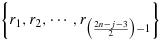
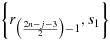
 , where K1 is a starting point and K2 is an ending point of a maximum walk in some S with a 2n × 2n area described in the previous section. In this section, we study all the basic properties of paths generated by straight and nonoverlapping walks by K(i,j). For the configuration explained in the first part of the proof of Theorem 3.3, we divide P1 into the following partitions:

 join the cells (2n − i − 1,j) to (2n,2n − 1), and the set of vertices {s1s2,⋯,sn + 8} join the cells (2n,2n) to (i,j + 1). The pairs of vertices {p(4n + 2),q1},{q(2j − 5),r1} and
 are also joined. The length of this polygon is
 (4.1)
(4.1)The properties of the positioning of K1 and K2, i.e., the number of columns and rows on the sides of K1 and K2 in S, in Theorem 3.3 still holds here.
Lemma 4.1.
 is rectifiable.
Proof.Since 4.1 is bounded for all the combinations of vertices joining the K1 and K2, the path f1 is rectifiable. (See 37 for rectifiable curves) □
Lemma 4.2.f1 is of bounded variation (BV) on [K1,K2].
Proof.We have

Theorem 4.3.Let f be a vector valued function defined as
 with components f = (f1,f2,⋯,fk), then f is rectifiable.
Proof.We have seen that f1 is rectifiable (see Lemma 4.1). Suppose
 . The graph of f2 is drawn differently than f1 in the sense that, joining seven vertices beginning from K1, we will arrive at the cell (2,3), and these seven cells are as follows:


Theorem 4.4.Suppose
 ,
,
 are all possible maximum walks in a 2n × 2n area (Ki need not be in an adjacent cell to Ki − 1). Suppose these paths are overlapped either partially or completely, but each path is continuous, then the vector f = (f1,f2,⋯,fk) is continuous.
Proof.Suppose f1 is a path which describes a walk from K1 to K2 and f2 is a path which describes a walk from K2 to K3 and so on, the piecewise combined paths are also continuous. Since each path component is also continuous, f is also continuous. □
Remark 4.5.By corollary 3.5, we have [2n{(2n × 2) − 2}] paths until all possible maximum walks of Theorem 4.4 are generated. We are interested in the investigation of properties of such walks. Whichever cell we initiate our walk from, all possible maximum distances are covered in the process of generation of f.
5 The open problem
Instead of constructing rectifiable paths by allowing a movement through adjacent rows and columns, here we allowed movements through adjacent diagonals as well. Such a construction will lead to multiple possibilities of maximum walks by starting at each cell, which we call trees of paths. Trees are formed at each cell whose branches are rectifiable paths. These trees, which are flexible and exhaustive, are helpful in visualizing more realistic chicken walks on square grids.
 (5.1)
(5.1) (5.2)
(5.2)If the walking path position at t1 is located in the first or last row or in the first or last column (except in the four corner cells), then there are four possible moves available to reach neighboring cells at time t2. At the next stage, i.e., at t3, we have at least six possible walking options for each of the seven previous positions in 5.2, unless at t3 we arrive at the first or last row or at the first or last column. Similarly, we can identify the number of possible options at each of the future time points. By connecting cells from the origin at t0 through each of the possible options at each of the time points, t1,t2,⋯, we will construct several rectifiable paths that have maximum distances covered. Can we obtain a generalized formula for the number of paths with maximum distances within S?
For example, for 3 × 3, we will have 16 maximum walks if a path is initiated at (3,3), 10 maximum paths for each walk if it is initiated at the first or last row or at the first or last column (except in the four corner cells) and six maximum paths for each walk initiated at corner cells, which gives a total number of paths with maximum possible distances in 3 × 3 area of 80. Two examples of maximum paths in the 5 × 5 grid are shown in Figures 11 and 12.


6 Discussion
Deconstructing movement into individual nonoverlapping walks within a grid-delineated area, which may then be strung together to model the frequently repetitive, overlapping walks characteristic of the domestic chicken, provides a framework to model fecal parasite dissemination. Under the straight and nonoverlapping setup, we are able to prove conditions that prevent formation of maximum walks in a 2n × 2n grid (see Theorem 3.3) and in a (2n + 1) × (2n + 1) grid (see Theorem 3.6). In section 4, we have proved that a vector of functions of BVs defined on a maximum possible walk is rectifiable. By joining several rectifiable paths, we arrive at more meaningful chicken walks, which mimic several realistic situations for understanding parasite transmissions. Incorporating data describing the rate of defecation (and thus parasite excretion) and previously modeled transmission rates will then be key components in the construction of pathogen transmission models. Here we describe a mathematical model defining host movement, in this case a chicken, but it could be any host, as the first tier of detail in the construction of a dynamic model for transmission of a pathogen which is usually not airborne, such as Eimeria. Spatial placement of a chicken in its pen or enclosure at any given time allows calculation of primary parasite dissemination, providing a tool with which the frequency of opportunities for neighboring naive chickens to become infected may be predicted. Extension of these calculations can be used to model pathogen transmission through a flock. This approach can be adapted with relevant biological parameters for any pathogen transmitted by direct or indirect physical contact.
We have provided a framework for understanding walks of chicken. By joining several nonoverlapping walks, we get one complete walk of a chicken per unit time. By joining several individual nonoverlapping walks, the resultant walk contains subwalks which could be overlapped, and this is close to the reality of a flock of birds in a pen. Since the size of a cell within a grid is arbitrary, our analysis is flexible to capture walks within very small pen sizes. Informed by this framework, each individual walk taken by a chicken may be portrayed across grids through diagonal as well as nondiagonal dimensions. By joining multiple paths, we can define possible chicken behavior over longer periods of time. Marrying these behavioral measures with biological data, including previously published rates of parasite transmission, we hope to develop a method of understanding pathogen transmission dynamics within the pens. One of our future aims of understanding chicken walks is to predict the presence or absence of Eimeria in a chicken and hence the proportion of infected chickens in a pen as an important step towards transmission dynamics models for Eimeria. We wish to study and build conjectures in general on association between the longest paths of bird movement and disease dynamics. Other potential applications for our chicken walk models include building age-structured graphical models for chicken walks.
Acknowledgements
Professor Lord Robert May (University of Oxford) encouraged new ideas introduced in this work to study bird movements and gave useful comments; Professor Tetali Prasad (Georgia Tech, Atlanta) suggested to draw figures in section 4; Professor Christopher Bishop (State University of New York) suggested key references on Hamiltonian path problems. Very useful corrections and comments by the two referees helped us to rewrite several sentences and to add section 2, which improved the overall content of the paper. Professor N. Yathindra (Director, Institute of Biotechnology and Applied Bioinformatics, Bangalore) and Professor N.V. Joshi (Indian Institute of Science, Bangalore) introduced Arni Rao to the Eimeria project initiated by the Royal Veterinary Collage, London. Our sincere gratitude to all. This work was funded by BBSRC (reference number BB/H009337/1).