

Analysis of Diffusion-Controlled Dissolution from Polydisperse Collections of Drug Particles with an Assessed Mathematical Model
Abstract
We introduce a “hierarchical” modeling strategy designed to be systematically extensible to increase the detail of dissolution predictions from polydisperse collections of drug particles and to be placed on firm mathematical and physical foundations with diffusion-dominated dissolution at its core to predict dissolution and the evolution of particle size distribution. We assess the model with experimental data and demonstrate higher accuracy by treating the polydisperse nature of dissolution. A level in the hierarchy is applied to study elements of diffusion-driven dissolution, in particular the role of particle-size distribution width with varying dose level and the influences of “confinement” on the process of dissolution. Confinement influences surface molecular flux, directly by the increase in bulk concentration and indirectly by the relative volume of particles to container. We find that the dissolution process can be broadly categorized within three “regimes” defined by the ratio of total concentration Ctot to solubility CS. Sink conditions apply in the first regime, when  . When
  (regime 3) dissolution is dominated by confinement and normalized saturation time follows a simple power law relationship. Regime 2 is characterized by a “saturation singularity” where dissolution is sensitive to both initial particle size distribution and confinement. © 2015 Wiley Periodicals, Inc. and the American Pharmacists Association J Pharm Sci 104:2998–3017, 2015
INTRODUCTION, MOTIVATIONS, AND BACKGROUND
Dissolution is a central element in the absorption of pharmaceuticals in the gastro-intestinal tract, beginning with gastric emptying and followed by the transport of drug particles along the gut, radial mixing within the gut, and the delivery of pharmaceutical molecules to the epithelium in preparation for trans-epithelial transport into the blood stream. For low solubility drugs, dissolution can be the rate-controlling step in this process. Furthermore, in vitro dissolution testing plays an important role in regulatory approval of new or changed products, and dissolution models are in the core of commercial systems-level software environments such as GastroPlus®, PK-Sim®, and Simcyp®. For these reasons, there is value in developing deeper levels of understanding of the dissolution process and its control, as well as in the development of more accurate mathematical models and methods to predict rates of dissolution. Given the small size of typical drug particles (<100 μm), and the frequent use of micronization of low solubility drugs, a dissolution model needs, at its core, an accurate diffusion-based model for dissolution from single drug particles.
In this paper, we build on a previous study that critically examined the accuracy of basic mathematical models built on solutions of the diffusion equation (i.e., “first principles” models) designed to predict the details of diffusion-dominated dissolution from single confined drug particles. Wang et al.,1 referred to as W12 in what follows, quantified and contrasted the accuracy level of physics-based mathematical models of diffusion-dominated single-particle dissolution in order to identify a first-principles model that balances accuracy with practicality of use. They found that a relatively simple “quasi-steady state” model (QSM) predicts both the increase in bulk concentration and the surface flux with high-level of accuracy beyond a short initial transient so long as effects of confinement are carefully included in the prediction. The QSM further provides an analytic expression for what W12 refer to as the “γ confinement effect,” one of two “confinement effects” discussed in detail in the current study. W12 show that this mathematical expression is accurate to within a few percent even with large relative γ confinement effect.
Since the QSM was found to be both practical and highly accurate for most applications, we place the QSM at the core of a strategy to predict dissolution from polydisperse collections of small drug particles of different size, as well as the change in particle size distribution with time for complete dissolution or saturation (“polydisperse model”). Accurate accounting for the confinement of dissolved concentrations of molecules by boundaries is treated with care. We present our polydisperse model strategy as the lowest level within a hierarchical building block framework in which the core physics-based model for normalized flux of drug molecules from particle surfaces (“Sherwood number,” Sh) can be generalized to include hydrodynamic enhancements, surface chemistry, particle geometry influences, and so on. The hierarchical formulation is developed in the next section preceding the mathematical formulation for the polydisperse model for diffusion-based dissolution from confined polydisperse collections of drug particles. The approximations made in the model are presented along with potential enhancements for future increases in complexity and generality.
We validate the model by comparing with experimental data and demonstrate the increased accuracy in predictions afforded by treating the polydisperse nature of particle sizes in contrast with a monodisperse representation. After validation, we apply the model in a detailed study of dissolution from polydisperse collections of drug particles in order to characterize the influence of the range of particle sizes on the dissolution process. We further evaluate and characterize the roles of confinement on dissolution and discover that the dissolution process, sensitivity to distribution width, and the role of confinement are characterized differently within three regimes that are defined by the nondimensional parameters  and
and  , where Ctot is total concentration, CS is solubility, and υm is the molar volume of the drug particles. We further show that by quantifying data from dissolution experiments in nondimensional form with specific nondimensional variables, the data can be generalized to describe multiple drugs.
Relationship to Previous Studies
A number of papers propose theoretical models to predict dissolution from polydisperse groupings of particles. Most of these apply a Noyes–Whitney type equation as a starting point, often generalized to include a specified “stagnant” or “diffusion layer” thickness. Dressman and Fleisher,2 for example, developed a mixing-tank model for predicting dissolution controlled oral absorption for a monodisperse powder using this kind of dissolution model. One of the earliest attempts at polydisperse models was developed by Higuchi and Hiestand3 using a simplistic approach with questionable assumptions such as fixed bulk concentration. The first true polydisperse model was developed by Hintz and Johnson4 who modified the Dressman and Fleisher approach to take into account the accumulation of molecules in the bulk fluid. In this and subsequent work,5-8 a diffusion-layer representation for single-particle dissolution was applied with an assumed form for diffusion-layer thickness.
The application of first-principle conservation laws to predict diffusion-layer thickness (in the form of Sherwood number) is central to the current work. A number of previous studies have applied Noyes–Whitney like models with diffusion layer thickness assumed to be constant, or heuristically specified with reference to experimental data. Examples include the studies by Simões et al.,9 Almeida et al.,10 Cartensen and Dali,11 Wang and Flanagan,12, 13 Shan et al.,14 Sheng et al.,15 and Johnson and coworkers.4-8 The latter works originate with Hintz and Johnson4 where the diffusion layer thickness (h) is assumed proportional to particle radius up to a maximum value above which h is held fixed at hmax. There was no first-principles basis for this assumption and hmax has sometimes been chosen so as to maximize the fit between a prediction and a dissolution measurement.5, 6 In other studies, the diffusion layer thickness has been taken to be constant and independent of particle radius and/or time.12, 13
An aim of the current study is to extend W12 to dissolution from polydisperse collections of particles in which diffusion thickness assumptions are replaced with an approach that has, at its core, the conservation law for diffusion dynamics, what is meant by “first-principles” modeling. As in W12, we argue that the treatments of “diffusion layer” thickness as a model constant should be avoided as this assumption is inconsistent with true dissolution physics. A difficulty has been lack of theoretical foundation built on first principles (i.e., the conservation laws)—a focus of the current hierarchical modeling strategy. Similarly, basic mechanisms surrounding the dissolution of polydisperse collections of drug particles are not well understood, another aim of the current work.
Another approach to modeling the evolution of polydisperse collections of particle sizes is the prediction of particle size distribution through a “population balance equation,” the evolution equation for the particle size distribution function. The population-balance method was first proposed by Shapiro and Erickson17 to model the combustion of sprays. This approach has been developed primarily in the chemical engineering literature in context with combustion processes. Examples include the work of Hulburt and Katz,18 LeBlanc and Fogler,19 Bhaskarwar,20, 21 Dabral et al.,22 Giona et al.,23 and Bhattacharya.24 For most conditions, the theoretical solution does not exist and the population-balance equation must be solved numerically. At the core of the population-balance equation is the dissolution of single particles in the distribution, and therefore the same need to model diffusion-layer thickness arises.
We apply the population balance framework in the current study, but with the work of Wang et al.1 at the center of a hierarchical modeling strategy built on first-principles dynamics. W12 derived an exact model for the details of diffusion-dominated dissolution from single confined particle and compared with a lower order QSM. They found the QSM to be highly accurate so long as confinement effects are properly taken into account. In the present work, we extend the single particle model developed in W12 and propose a new polydisperse model with the more accurate estimation of diffusion layer thickness.
MATHEMATICAL MODEL FORMULATIONS
A General Framework for Dissolution from Polydisperse Collections of Drug Particles
We develop a mathematical modeling framework for accurate predictions of dissolution from polydisperse collections of drug particles designed so that geometric, hydrodynamic, and chemical complexity can be progressively enhanced through a hierarchical modeling strategy in which complexity increases with level in the hierarchy, or where specific physical effects may be included or excluded depending on application. Because of the small size of typical drug particles and the current trend toward micronization, the mass flux from the particle surface is largely driven by molecular diffusion. Therefore, at its core, the framework contains an accurate model for diffusion-dominated dissolution from single spherical particles. The concept of a hierarchical framework is a modeling structure where the diffusion-based core can be systematically enhanced to include effects that alter diffusive transport from spherical particles. Relative motion between the particle and solvent, for example, increases surface flux by convection; pH surface chemistry can alter surface flux; nonspherical particle geometry, agglomeration, and deagglomeration can alter net dissolution rate relative to pure diffusive transport from a spherical particle.
Dissolution generally involves flux and dispersion of drug molecules from large collections of small particles of different size and shape. Our hierarchical strategy centers on progressive enhancement of a single-particle diffusion-dominated core within a generalized model for polydisperse collections of particles of different size. The mathematical structure of the polydisperse model predicts the change in the distribution of particle sizes over time from an initial specified particle size distribution. The central model assumption is that the particles, and the local bulk concentrations around the particles, are homogeneously distributed over the volume that confines the particles (the “container”). Useful future model enhancements could include the possibility of nonuniform particle distributions and local bulk concentrations, particle-particle interactions, agglomeration/deagglomeration, and so on. In addition, although we develop here a model for the release of pharmaceutical molecules into a medium confined by an impermeable container such as the United States Pharmacopeia (USP)-II in vitro dissolution device, a future enhancement useful for in vivo dissolution will include absorption at container surfaces and permeability models.
Normalized Surface Flux (Sh) and the “Diffusion Layer” (δ)
 (1)
(1) (t) is the average flux of molecules (moles/time/area) from the particle surface into the bulk fluid,
  is the concentration of molecules (moles/volume) at the particle surface,
  is the average concentration of molecules in the “bulk” fluid surrounding the particle and confined by a “container” (moles in the bulk fluid divided by bulk fluid volume),
  is the diffusivity of the molecule in the medium and
  is the particle radius at time t (if the particle is not spherical, R is “effective” particle radius). Although the term “Sherwood number” suggests a single value, Sh should be recognized as a normalized flux that varies from particle to particle and changes with time. Pharmaceutical molecules are released into the bulk in concert with reduction in particle radius, so
 and are both strong functions of time. The surface concentration, however, is driven by the surface kinetics. In the current model, we assume diffusion-driven dissolution and apply the common assumption that the fluid adjacent to the surface is saturated with surface concentration CS given by the solubility of the drug molecule in the medium, a fixed value.
 (2)
(2) ). As illustrated in Figure 1, Eq. 2 defines δ by extrapolating the
  concentration with a straight line from the particle surface with the true slope
  at the particle surface. The distance where this linear extrapolation crosses the bulk concentration
  is δ, a quantification of the thickness of the concentration layer adjacent to the particle surface. We shall return to Eq. 2 and Figure 1 later in our discussion of confinement effects.
Single Particle Dissolution
 . The rate of change in radius is determined by the rate at which molecules leave the particle surface and enter the bulk fluid surrounding the particle:
 (3)
(3)The concentration of molecules in the bulk fluid,  , is obtained by integrating Eq. 3 to obtain the change in radius (and volume) for each particle in the collection from time step
  to
to  and the loss of particle volume
  is converted to the addition of
  molecules to the bulk fluid (
 ) from which the new number of molecules in the bulk
  is obtained at the next time step and the bulk concentration
  is recalculated, a step that depends centrally on the confinement of the molecules in the bulk volume,
  . The updated value for
  is then incorporated into Eq. 3 at the next time instant and the calculation is continued forward in time. Thus, the accuracy of the predictions for the release of molecules into the bulk from the surfaces of collections of particles depends on the accuracy of the model for
  for each particle in the collection (see section A Polydisperse Hierarchical Model for Diffusion-Dominated Dissolution below). The time change in particle bulk concentration,
  , is strongly dependent on the confinement of the released molecules by the container into which the molecules are released. As discussed in the next section, this is one of two “confinement effects.”
The Core Single Particle QSM
Wang et al.1 showed that the QSM is both accurate and practical for predicting diffusion-driven dissolution from single spherical particles of volume  confined by a spherical impermeable container of volume
  . This is a first-principles model based on the diffusion equation (Ficks second law) and applied to dissolution from a particle with the essential approximation that the nonsteady term in the equation is negligible. This is true when time is large compared with the diffusion time scale,
  —which, for dissolution from small pharmaceutical particles, tends to be very short compared with the time required for measurable change in bulk concentration. W12 showed that the QSM is an excellent approximation for predicting the time changes in bulk concentration
  because the error in neglecting the nonsteady term in the model for normalized surface flux
  when Eq. 3 is integrated in time occurs largely during the initial period of dissolution when the concentration field is first developing and Cb is very small compared with CS, so the error in the prediction of surface flux occurs when there is little measureable effect on the bulk concentration.
The QSM therefore predicts  accurately so long as the confinement of molecules added to the bulk fluid in
  is accurately incorporated into in Eq. 3 in
  as described in the paragraph above. The restriction of molecules to the region between the particle and container leads to a second “confinement effect” for which the QSM produces a very useful and accurate explicit mathematical expression (W12).
 at infinity and then adjusting
  to be consistent with the concentration field confined to a volume,
 . The steady form of the diffusion equation with the requirement that the concentration at the particle surface and infinity are CS and
  is easy to integrate, to produce:
 ()
() ()
() in Eq. 4a to make the volume integral of
  over the container volume
  equal total number of molecules that have been released into the container to time t. Integrating
  over the volume between the particle and container surface and dividing by the bulk volume
  produces the required relationship between
  and
and  (see W12):
 (5)
(5) (6)
(6) replaced by Eq 5. Equating this QSM prediction for flux with the general expression for flux given by Eq. 3 produces the QSM prediction for Sh, the normalized flux of molecules from a particle of volume
  in a container of volume
  :
:
 (7)
(7)Thus, in diffusion-driven dissolution, the normalized flux is dependent only on the relative volume of particle to container. When the container is sufficiently large compared with the particle, or the particle is sufficiently small compared with the container, that  and Eq. 6 gives
  , Eq. 7 gives Sh ≈ 1. Thus, γ results from the influence of confinement of molecules in the “container” surrounding the particle on the rate of dissolution from a single particle. The second term in Eq. 7 is a modification to the Sherwood number from confinement that results from the solution of the diffusion equation. W12 have shown that this additional term is a very close approximation of the exact term calculated from an exact solution of diffusion-driven dissolution from a spherical particle in a spherical impermeable container. γ underlies a second confinement effect mentioned above and discussed in detail in the section Regimes that Define the Dissolution Process and Confinement below.
The Hierarchical Particle Dissolution Model
 or : at each instant in time the diffusion layer thickness equals the particle radius. However, Eq. 7 shows that Sh is increased above one by the confinement of molecules within a finite volume
  . In addition, Sh can also be enhanced by flow, for example, by relative motion between the fluid and the particle surface (“slip”) enhancing mass transfer at the surface by convection. Thus, in our hierarchical modeling framework, we write, for each particle,
 (8)
(8) (9)
(9)It can be shown from Eq. 6 that  , so that
  . Thus, the “γ confinement effect” has the potential to be significant.
Equation 3 with Eq. 8 are at the core of our hierarchical model strategy. However, to represent realistic drug dissolution, the model must be extended to include polydisperse collections of small drug particles of different size. In the current study, we analyze diffusion-dominated dissolution, so  (QSM) as per Eq. 7.
A Polydisperse Hierarchical Model for Diffusion-Dominated Dissolution
To place Eq. 3 with Eq. 8 at the core of our polydisperse model, consider a collection of particles of different sizes distributed uniformly within a container of volume Vc as illustrated in Figure 2. Here, Vc is the volume of the entire container in which are contained particles  of radius
  . The total number of particles,
  , changes with time as the dissolution process proceeds. However, because the particle surface fluxes are local maxima, at each time t there exists a closed surface around each particle across which the flux of molecules is zero. Therefore, each particle j is surrounded by an “effective particle confinement volume”
  that changes with time as the particles reduce in size. Assuming that the surrounding container volume is either fixed or changes slowly relative to the rate of dissolution, the time scale governing the rate of change in
  is commensurate with the time scale for the rate of change in particle radius, so that, according to the quasi-steady-state approximation, the time rate of change of
  can be neglected in a polydisperse particle dissolution model, to a good approximation.
  varies from particle to particle, locally confining the accumulation of molecules around each particle at each instant in time.

 at time t:
 (10)
(10) (11)
(11) is the radius of the particle with volume
  . Note that in the third equation of 11, the “container volume” of Eq. 6 is now the “effective particle confinement volume”
  surrounding particle j, as discussed above. Similarly,
  in Eq. 3 is replaced by
  , the bulk concentration of molecules in the effective particle volume
  surrounding particle j. In using Eqs. 10 and 11, we model the particle as spherical in a spherical confinement volume. Future improvements on these two model approximations are possible. However, more important is that Eq. 10 is extensible as per Eq. 8 in a hierarchical modeling framework to include enhancements to the dissolution rate from effects other than diffusion.
Although the individual particle confinement volumes change with time, at each time t the sum of particle confinement volumes must equal the total container volume:  . In the current application of the model to in vitro dissolution (e.g., the USP II device), the container volume Vc is fixed during the dissolution process. However, Vc could vary with time, as would be the case in vivo when the “container” is interpreted as a pocket of fluid confined by a localized contraction within the small intestine.
The aim of our model is to accurately predict three characteristics of the dissolution process: (1) the time evolution of the distribution of particle sizes,  ,
, ; (2) the rate of release of molecules into the bulk fluid of volume
  at each time t; and (3) the time change in bulk concentration in the container volume
  , that is,
  , where
  is the number of pharmaceutical molecules in the bulk fluid surrounding all particles within the container. We will find that the predictions for time required for complete dissolution or saturation will form the basis for discussing fundamental differences in dissolution physics within section Regimes that Define the Dissolution Process and Confinement (below).
Evolution of the Particle Size Distribution
Consider the sudden mixing of a known distribution of spherical pharmaceutical particles in a liquid medium confined to an impermeable container of volume Vc. Diffusivity and solubility are assumed known at required levels of accuracy. As mentioned previously, we assume that the fluid adjacent to the particle surfaces is saturated with concentration equal to the measured solubility. Dissolution begins at time  assuming no molecules initially in the bulk fluid surrounding the particles.
 , so that
  . Let N(t) be the total number of particles at time t, so that
  is the number of particles between R and
  . Thus,
 (12)
(12) is the number distribution function. The aim is to
  predict, from which the change in volume of all particles, the number of molecules introduced into the bulk and the bulk concentration are determined as a function of time.
 written in terms of
  with the time rate of change of particle radius
  between R and
  , the differential equation for the time evolution of the particle distribution
  function can be derived20:
 (13)
(13) depends centrally on the accuracy of the model for rate of change of particle radius
  for each particle j in the polydisperse collection, as given by Eqs. 10 and 11 above. From the solution
  for,
for, 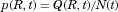 is easily determined, as is the total volume of particles,
  :
:
 (14)
(14) , it is now possible to calculate the number of molecules in the bulk fluid, and therefore the bulk concentration:
 (15)
(15)Equation 13 with Eqs. 10 and 11 must be solved on the computer to obtain the number distribution  discretized in R and t from a specified initial distribution
  . Typically,
  must be obtained from measurements of particle volume fraction distribution using an instrument such as the Mastersizer (Malvern Instruments). Furthermore, to predict
  Eq. 9 a model is needed for the effective container volume
  surrounding each particle. These issues are discussed next.
Computation of the Particle Distribution Function Equation
Starting  with, we solve Eq. 13 with Eqs. 10 and 11 in discretized form.
  is discretized as a function of discrete particle radii
  and over discretized time steps
  , where j and n are positive integers. There are at least two approaches to solve for
  discretized. The first is to discretize Eq. 13 using finite differencing in R and t and advance the discretized equation in time for
  directly, with
  replaced by the QSM Eqs. 10 and 11 at time tn. The second approach is to solve Eq. 13 indirectly by discretizing
  into bins
  of fixed radius
  at
at  and then integrating
  from the QSM Eqs. 10 and 11 to obtain
  at the next time step. The number of particles
  in each bin
  is fixed as the radii of each bin decrease with time and the particles in that bin dissolve and are removed from the distribution. Thus, as the change in bin sizes
  are calculated along with particle radii
  from Eq. 10, the change in discretized
 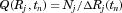 with time is determined. We found that the first approach was prone to numerical instability, so we used the second approach, which is similar conceptually to the algorithms described by Hintz and Johnson4 and Lindfors et al.25 that did not include Eq. 13 as the mathematical basis for prediction of time evolution of particle size
  distribution. Furthermore, to integrate the QSM Eqs. 10 and 11, an “effective particle volume” must be quantified. This is described next.
The “Homogeneously Mixed” Model Assumption
As pointed out above, we differ from previous approaches in the hierarchical approach taken and the use of the QSM at the core of our polydisperse dissolution model. Here, we consider confined dissolution by pure diffusion: the first two terms in Eq. 8 with Eq. 9 (or equivalently, Eq. 11). As discussed above, the second term in Eq. 8 (or 11) is a confinement effect for a single particle j in its effective confinement volume  . The model used to determine
  is an issue worthy of discussion and refinement in future application of in the polydisperse dissolution model. In the current implementation, we apply the “homogeneously mixed” model assumption where the particles in each
  bin are assumed to be homogeneously distributed within the container volume Vc, and each effective confinement volume is assumed to have the same bulk concentration. That is, in our current model we assume that
  is the same surrounding all particles j at each time t, although the net bulk concentration
  varies with time.
This “homogeneously mixed” model assumption is effectively the same at that assumed by Hintz and Johnson4 and Lu et al.5 and is an element that should be refined in future models to take into account inhomogeneous concentrations of molecules in the bulk fluid, as is likely the case with in vivo dissolution in the gut.
The Initial Number Distribution Function
As described above, to initiate the calculation of  the initial distribution
  must be estimated from measurements or must specified ad hoc. For example, in experiments developed by Weibull26 and reported in W12 and Lindfors et al.16 the Mastersizer instrument was used to measure the volume fraction of particle sizes within logarithmic bands of particle radii as illustrated in Figure 3. From the initial total volume of particles
  , the total concentration
 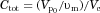 may be calculated.

 form, let
  be the volume fraction in bin j given as output from the Mastersizer and displayed in Figure 3. Thus, by construction,
  . For each bin from
  to
to  , it is straightforward convert to bin widths on a linear scale (i.e., bins from
  to
to  ). Note that
 (16)
(16) and
and 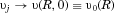 , so that Eq. 16 becomes:
 (17)
(17) is the volumetric probability distribution function at the initial time and
  is the fraction of volume of the particles between R and R + dR at t = 0. Thus
 (18)
(18) is the total volume occupied by the particles at the initial time,
  is the volume distribution function, and
  is the volume of particles between radii R and
  .
. is the particle distribution function
  multiplied by the volume of a particle with radius R, so that
 (19)
(19) and N0 are the PDF and number of particles at t = 0. Thus, the method to find
  from the Mastersizer outputs of logarithmically discretized volume fraction
  and total number of particles N0 is as follows:
 Form,
Form, at the desired particle radii R at whatever resolution is desired,
 (and
(and  ) at the desired resolution.
In our computational experiments (below), we discretized R into 500 bins bounded by discretized radii values  .
.
Generalized Distribution Functions and Average Particle Radii
 , they actually apply at arbitrary time, t. Thus, as the time evolution of the particle number distribution function
  is obtained by integrating Eq. 13, so are the distribution
  functions,
  from Eq. 19, and
  . A similar process can be used to define the surface probability distribution function
  and surface distribution function
  , where
  is the total surface area of all
  particles at time t, and
 (20)
(20)
Thus, from a prediction  of, one can also construct, at each time t, the surface and volume probability and distribution functions,
  and
and  , as well as the total number of particles
  , the total volume of particles
  , and the total surface area of particles,
  .
.
 . However, this definition is not unique and one might also consider average radius based on the volume or surface area of the particles. Each of these definitions can be constructed from the prediction for
  by constructing the number probability distribution function p(R,t), volume probability distribution
  function, and surface probability distribution function
  and using the averaging property of the pdf:
 (22)
(22) (23)
(23) (24)
(24)Thus, from the prediction of the number distribution function  most other quantifications of interest can be made. In our computational experiments (below), we show the differences in evolution of average particle radius using the three definitions above.
COMPUTATIONAL EXPERIMENTS
Model Assessment
Model predictions in which the polydisperse particle size distribution is approximated by particles of a single size (monodisperse) are common in current prediction approaches. It is therefore relevant to ask: 1 Does the additional complexity of the polydisperse model above produce accurate predictions for realistic dissolution scenarios? and 2 Does the additional complexity embedded in the modeling of distributions of particle sizes significantly improve the accuracy and generality of the predictions in comparison with monodisperse treatments? These two interrelated questions are addressed in this section, with the latter question the subject of more detailed analysis in following sections.
Wang et al.1 compared predictions of monodisperse collections of particles, where the single particle radius was equal to the volume-averaged radius of the polydisperse collection, with experimental measurements of dissolution from polydisperse collections of felodipine drug particles in a Couette flow viscometer. The experiments were carried out by Weibull26and also described by Lindfors et al.16 Felodipine is classified as a Biopharmaceutics Classification System II drug with extremely low solubility. In the experiments described by Lindfors et al., solubility is CS = 0.89 μM (0.34 μg/mL), molar volume is  and diffusivity is
  . Felodipine has a molecular weight of 384 g/mol.
 , where
  is the total number of molecules in the (fixed) container of volume
  . As pointed out by W12,
 (25)
(25) ). W12 showed that the absolute bulk concentration with time,
  is not well predicted by the monodisperse model. However, the relative bulk concentrations in the two predictions due to the different levels of confinement of drug within the in vitro dissolution device, quantified by Eq. 25, were accurately predicted, demonstrating the importance of including confinement in predictions as molecules accumulate in the bulk.
The details of the experiments are described in Lindfors et al.,16 Weibull26 and W12. A simple laminar shear flow with closely linear velocity profile was created by rotating the inner cylinder of a Couette viscometer at 5 rpm, producing a low Reynolds number laminar flow that, together with the small size of the particles (3.34 μm average diameter), produced highly diffusion-dominated dissolution from non-aggregated particles, made neutrally buoyant by density-matching the aqueous medium. The initial particle size distribution measured with the Mastersizer instrument is given in Figure 3; the radius at the peak in the volume–fraction distribution is  .
.
In Figure 4, we compare the experimentally measured increase in bulk concentration from the Lindfors et al.16 experiment with predictions using monodisperse and polydisperse models with the QSM at its core as described above. For the polydisperse model predictions, we initialize the calculation with the size distribution obtained by the volume fraction in Figure 3. For the monodisperse model predictions, we use the volume average radius measured by Lindfors et al.16 (R = 1.67 μm). Consistent with Figure 2 in Johnson,7 Figure 4 shows that taking into account the polydisperse nature of particle size corrects the errors in the predictions of bulk concentration using the monodisperse model at both Ctot values. The improvement is particularly apparent during the initial period of dissolution where the initial rapid dissolution from the smallest particles is accurately captured with the polydisperse particle model but is not properly treated by a monodisperse model with only single particle radii.

After the smaller particles have mostly dissolved, the dissolution process enters into a final dissolution period that is dominated by the release of molecules from the largest particles in the distribution. From Eq. 9, dissolution rate is proportional to  , slowing over time as molecules entering the bulk are confined by the container. In contrast with the initial period where the smallest particles must be represented to accurately predict dissolution, Figure 4 shows that in the later period accurate prediction of this process requires a polydisperse model to capture dissolution from the largest particles. Note, specifically, that when
  , the single particle size model predicts saturation at about 250 min, whereas the polydisperse model takes into account the much longer time required for the larger particles to dissolve.
We conclude that treating the true polydisperse nature of particle size distributions in dissolution dynamics produces potentially useful details that are outside the capability of monodisperse models.
Sensitivity to Initial Particle Size Distribution
Having validated the polydisperse model, we apply the formulation in a series of computational experiments to study characteristics relevant to diffusion-dominated dissolution of large collections of small drug particles in impermeable containers. Our aim is to provide useful insight from quantifications of the sensitivities between the dissolution process, the range of particle sizes in the initial distribution of particles, and the total concentration of drug molecules in the container ( ). In this section, we explore the role of the range of particle sizes to details of the dissolution process. In following sections, we provide new understanding of the subtle role of confinement and the “saturation singularity” on the dissolution process.
Specification of Initial Particle Size Distribution
To systematically vary the initial distribution of particle sizes, the initial size distribution should be specified in a form consistent with true distributions. As illustrated in Figure 3, realistic size distributions are typically well-represented as Gaussian functions of the log of the particle radii  (log-normal). For our computational experiments, we therefore initiate our simulations with a log-normal volume fraction distribution
  similar to Figure 3, but much more finely resolved in
  (500 vs. 22 bins). For our results to be more generally applicable to a wide variety of particle sizes, we specify the distribution relative to nondimensional particle radius, where R is nondimensionalized by the radius at the peak in the distribution
  so that
 peaks at. The width of the distribution of particle sizes is correspondingly specified in terms of
  as illustrated in Figure 5a.

 is proportional to the initial volumetric probability distribution function,
  , so that
 (26)
(26) is the volume fraction
  of the total volume
  of the particles in the logarithmic band from
  to
to  . The logarithmic band-widths
  are specified as uniform in
  ; both
  and
and  peak
peak  at. To approximate measured particle distributions such as Figure 3, for example,
  is modeled as Gaussian in
  :
:
 (27)
(27) over
over  is unity as required by definition. (Note that
  varies from −∞ to +∞ as
  varies from 0 to ∞.)
  in Eq. 27 is symmetrical about the peak
  with its width controlled
  by, the variance of
  over
over  . Inserting Eq. 27 into Eq. 19 produces
  , the initial condition which is used solve for
  and, from that solution, all other needed quantities during the dissolution process, as described above.
Figure 5 shows the two initial conditions for  that were applied in the current study, a “narrow” distribution (N) with
  and a “wide” distribution (W) with
  . In both distributions, 500 logarithmic bins were used so that the bin widths were smaller with the narrow distribution than the wide. All particles in the same bin have the same radius and the bins farthest from the peak
  have volume fraction 0.001. These “farthest” bins are at
  for the narrow distribution and
  for the wide distribution. In Figure 5a, the volume fractions are given on a logarithmic scale. The corresponding initial pdf
  , plotted on a linear
  scale, is shown in Figure 5b. Because of the functional relationship between
  in Eq. 19, the PDF peaks
  at and the distribution exhibits a tail typical of manufactured formulations (e.g., Fig. 3). As the width of the distribution decreases, the dissolution process approaches that of a monodisperse distribution with single particle radius.
Effect of Initial Size Distribution on Drug Release
 , all at the same total concentration,
  . The evolution of bulk concentration
  varies with solubility CS, diffusivity Dm, molar volume υm, and the initial radius at the center of the volume fraction distribution,
  . However, it can be shown (see section Generalized Dissolution with Appropriate Nondimensional Parameters below) that all variations can be represented as bulk concentration nondimensionalized by the solubility (
 ) against time nondimensionalized by the following time scale:
 (28)
(28) is the time it takes for a single particle of initial radius
  to completely dissolve in an unbounded medium (with no molecules initially in the bulk). This is obtained by integrating Eq. 3 from
  at
at  to
to  at
at  with
with  and
and  .
.Thus, in what follows a plot of dimensional bulk concentration versus time can be obtained from a plot of nondimensional  against
  by forming
  from Eq. 28 and multiplying
  by CS and
  by
by  . Unless otherwise indicated, we use the properties of felodipine in the experiments of Lindfors et al.16 as given in section Model Validation above. However, as will be explained in more detail in the subsection below entitled Generalized Dissolution with Appropriate Nondimensional Parameters, when plotted and interpreted in proper nondimensional form, dissolution predictions are independent of drug properties.
In Figure 6, we plot the nondimensional changes in bulk concentration with respect to time initialized with wide (W), narrow (N), and monodisperse (M) distributions of drug particles at three total concentrations Ctot, one below the solubility and two above (CS = 0.89 μM). Three manifestations of confinement are immediately apparent. The first is the occurrence of saturation when confined and total concentration exceeds solubility. The second is the sensitivity between the rate of change in bulk concentration and total concentration Ctot which, as shown by Eq. 25 and discussed in W12, quantifies the relative confinement of particles in the container at the initiation of dissolution. A more subtle manifestation is that complete dissolution ( ) requires times longer than the unbounded dissolution time,
  . As Ctot decreases, dissolution time approaches
  , however at Ctot = 0.5 μM (Ctot/CS = 0.56), the time to complete dissolution greatly exceeds the unbounded domain dissolution time. We shall return to this issue in the subsection below entitled The γ versus Cb Confinement Effects.

Figure 6 shows the effects of particle distribution on the dissolution process. Not surprisingly, as the distribution narrows, the dissolution process approaches that for a monodisperse distribution of particles. However, the existence of a distribution of particle sizes lengthens the time required for complete dissolution or saturation to occur. This is because particles larger than  are the last to dissolve and do so in the presence of lower driving potential,
  (Eq. 10). Thus, although the narrow particle distribution closely approximates monodisperse dissolution at early times (Fig. 6b), the sensitivity to the existence of distributions of particle sizes is stronger in the final period of dissolution or saturation (Fig. 6a). The total time to dissolution or saturation is higher with a distribution of particles (at the same Ctot). We shall find that this is particularly true in the final periods of dissolution (
 ) as the final period is dictated by the dissolving of the largest particles.
Interestingly, although the rate of increase in bulk concentration is overall reduced by the existence of a range of particle sizes, the rate of increase in bulk concentration is initially increased because of the existence of a distribution of particle sizes. This is because the initial rate of increase in bulk concentration is dominated by dissolution of the smallest particles. It can be shown that the relative rates of addition of drug molecules to bulk concentration from groupings of drug particles with average radii  and
and  is proportional to
  , where
  and
and  are the contributions to total concentration from the first and second groupings of particles. Thus, the smaller particles are highly favored to contribute to the bulk concentration at a faster rate so long as the contribution of each group of particles is not correspondingly out of balance. As indicated by Figure 5b, the log-normal distribution biases the number of particles to sizes smaller than the most probable. As a result, the smallest particles initially dominate the rate of increase in bulk concentration. Figure 6b shows that the cross over in the rate of increase in
  between polydisperse and monodisperse collections of particles occurs at later time with larger Ctot.
Similar characteristics were observed in Figure 4 when we compared data from an in vitro dissolution experiment with predictions using a monodisperse model versus predictions using the true initial polydisperse distribution of particle sizes. Clearly there exist potentially important details of the dissolution process that cannot be captured with a monodisperse model.
The time variations of total number of particles N(t), normalized by the initial number of particles, is shown in Figure 7 for different total concentrations and distribution widths. We observe a great sensitivity both to the total concentration and to the width of the size distribution of particles. Because the rate of change in particle radius is inversely proportional to particle radius (Eq. 10), the smallest particles reduce in radius at the most rapid rate. With both “wide” (W) and “narrow” (N) distributions, there is an initial period with no reduction in particles, as the smallest radius group dissolves. Because the wide distribution contains the smallest particles (relative to R*), the time period before particle numbers begin to reduce is shorter, and the relative change in number of particles is initially most rapid, with the wide distribution, at all Ctot. With complete dissolution (Ctot < CS) the number of particle drop to zero; saturation (Ctot > CS) implies that some particles never dissolve. With increasing confinement (increasing Ctot) the rate of reduction in particles is lower and, with saturation, the number of retained particles higher. The largest particles in the initial distribution are the last to dissolve or saturate.

Evolution of Particle Size Distribution
Over time, the smaller and larger particles decrease in radius at different rates (Eq. 10) and the shape of the particle size distribution changes as drug molecules are released into the bulk. The changes in particle size distribution for the six simulations in Figures 6 and 7 using the wide (W) and narrow initial distributions of Figure 5 are shown in Figure 8, where for each case the number distribution function  is plotted at nondimensional time increments
  over the dissolution process for the three values of Ctot.

The distribution of particle sizes changes differently during dissolution depending on the level of confinement (υmCtot) and the width of the initial distribution. When Ctot is below the solubility (CS = 0.89 μM), all particles eventually dissolve and  (Figs. 8a and 8b), whereas for Ctot > CS, the dissolution process ends in saturation (Figs. 8c–8f). In all cases, the distribution of particle sizes is very different toward the end of the dissolution process in comparison with the initial distribution. In particular, because the rate at which the particle radius decreases is inversely proportional to the particle radius (Eq. 10 with Shj ≈ 1), the smallest particles in the distributions decrease in radius much more rapidly than do the largest particles, with the consequence that the distributions initially increase in width with time as the distribution rapidly extends towards zero radius. This initial increase in distribution width as the distribution extends in smaller radii is clear in all cases shown in Figure 8.
A consequence of the initial spreading of the distribution function toward smaller radius particles is that, over a period of time after the start of dissolution, the radius at the peak in the particle size distribution, Rpeak, shifts to smaller values. The initial time period over which this shift in Rpeak with time occurs depends on the initial width of the distribution and on Ctot and its value relative to CS. The radius at the peak in the distribution either asymptotes to its smallest value or it shifts back toward larger values until complete dissolution of saturation occurs. In particular, when dissolution begins with an initially “narrow” distribution, the radius at the peak in the number distribution shifts continuously toward smaller Rpeak until all particles have dissolved (Fig. 8a) or saturation has occurred (Figs. 8c and 8e) because the particle size is distributed in a sufficiently narrow region to approximate that from a monodisperse distribution—where all particle reduce together continuously to smaller values.
In contrast, the radius at the peak of an initially “wide” distributions decreases at first, but eventually shifts from decreasing to increasing Rpeak at a point in time that depends on Ctot (Figs. 8b, 8d, and 8e). As with all distributions, the initial shift in Rpeak to lower values results from the  (Eq. 10). However, as the smallest particles move to zero radius, they begin to dissolve and disappear from the distribution. When this occurs, the distribution is anchored at R = 0, whereas the largest particle continue to reduce in size and the change in distribution with time is dictated by the rate of change in radius of the larger particles. If the distribution is sufficiently wide and the dissolution process is sufficiently long, particle numbers accumulate rapidly at the smallest scales as particle numbers decrease at the largest scales, with the consequence that the peak in the distribution shifts towards larger scales.
It should be noted that a plot roughly similar to Figure 8d is given in Johnson8 (their Fig. 2), although the conditions under which the simulation is performed are not given. Likely because the bin resolution is much cruder than in Figure 8 and the largest particles did not appear to reduce in diameter in their simulation, Rpeak in their simulations moved rapidly to larger values. In contract, Figure 8 indicates that Rpeak initially decreases as the smaller particles rapidly reduce in size and dissolve, before sometimes increasing as saturation is approached, depending on the initial width of the distribution. Still, the essential mechanism is similarly described.
Changes in Average Particle Radius
The changes in radii at the peaks in the particle size distribution to smaller or larger values result from the differential rates of change of larger versus smaller particles (Eq. 10) in relationship to the total concentration of molecules available for dissolution relative to the saturation concentration (Ctot/CS) and the size of the container (υmCtot). These changes are reflected in corresponding changes in average particle size during dissolution, as shown in Figure 9 where average particle radius is plotted against time using the three definitions for average radius given by Eqs. 22–24 and, in each case, comparing with the continuous reduction radius with an initially monodisperse collection of drug particles. We find that all definitions produce the same trends and that these trends follow the evolution of Rpeak with time just discussed: the initially “narrow” distributions follow approximately the continually decreasing average radius of dissolution from the monodisperse collection, whereas the average particle radius with the initially “wide” distribution ultimately increases over time.

However, the initial reduction on average particle radius is observed only with the number-averaged radius. Neither the volume-averaged nor the surface-averaged definition for average particle radius is sensitive to the initial decrease in the peak in number distribution function shown in Figure 8. Furthermore, as the width of the initial particle size distribution increases, so does the difference between number-averaged radius, volume-averaged radius and surface-averaged radius. In fact, the volume-average radius can be a factor of two larger than the number-averaged particle radius with the “wide” distribution as volume-averaging weights the average toward the largest particles. Furthermore the proper representation of the polydisperse nature of the dissolution process has a large impact on predictions of time evolution of average particle size during dissolution. The improved accuracy in the prediction is particularly apparent when the particle distribution is relatively wide. In this case, average particle size increases over time, while the monodisperse model can only predict reductions in particle radius.
Interestingly, when Ctot < CS and all particles ultimately dissolve, the final period of dissolution occurs with minimal change in bulk concentration (Figs. 9a and 9b). This results because as particles accumulate near zero radius in the distribution, the relative number of molecules in these near-zero radius particles becomes so small relative to the total number of molecules in the bulk that the bulk concentration changes very little at the end of the dissolution process. Consequently the average particle radii in Figures 9a and 9b drop rapidly to zero at the highest bulk concentration as the final particles completely dissolve.
CONFINEMENT EFFECTS
 (Eq. 2). In effect, “confinement effects” alter the flux at which molecules leave a particle surface by altering the gradient in concentration at the particle surface (Eq. 3 with Eq. 10:
 (29)
(29) is the Sherwood number for particle j for diffusion-dominated dissolution based on the solution of the diffusion equation.
  is an enhancement that depends on
  , the volume of the particle relative to the effective volume that surrounds the particle and confines the release of molecules (Eq. 11). Equation 29 incorporates the “homogeneously mixed” model approximation (see section A Polydisperse Hierarchical Model for Diffusion-Dominated Dissolution).
Reference is commonly made to “sink conditions,” which implies that the dissolution process is well approximated as taking place with negligible effects of confinement so that Cb in Eq. 30 may be neglected relative to surface concentration CS. However, it is the existence of confinement that allows the average concentration within the “container”  to increase with time, forcing progressive reductions in the driving potential
  between the particle surface and bulk concentration and, equivalently, the gradient in concentration at the particle surface and the flux of molecules into the bulk. Dissolution stops then when the driving potential approaches zero. Although the approach to saturation is a clear manifestation of confinement, we show below that the influence of confinement on the driving potential becomes significant even when
  and saturation never occurs (see section Regimes that Define the Dissolution Process and Confinement).
The γ Confinement Effect
 for a significant number of particles in the collection. As given by Eq. 11, γj is an increasing function of the particle confinement ratio
  . For dissolution from polydisperse collections of drug particles, the average particle confinement ratio is the ratio of total particle volume to the volume of the impermeable container in which dissolution takes place. Clearly the γ confinement effect is strongest at the initiation of the dissolution process, when
  is largest and is proportional to total concentration:
  , where υm is the molar volume. In in vitro experiments, it is generally the case that
  so that the γ confinement effect near the initiation of dissolution can be well approximated by
 (30)
(30) (31)
(31) and Sh in Eq. 29.
In Figure 10, the average Sherwood number of felodipine particles is plotted against total concentration relative to the solubility using the polydisperse model described here with the QSM at its core. By comparing with the exact solution, W12 showed that the QSM produces a highly accurate prediction of  , so that the predictions in Figure 10 may be interpreted with confidence. The figure suggests that for felodipine a 10% effect requires Ctot/CS ∼ 1000. However, this result is for an exceptionally low solubility drug (CS = 0.89 μM). In Figure 10, we plot for the monodisperse case the γ confinement effect curves for drugs with
  10 and 100 times larger than felodipine. Ibuprofen, for example, has
  375 higher than felodipine and the 10% γ effect occurs when Ctot/CS is much lower, ∼2.7.
Furthermore, Figure 10 is an average; the γ confinement effect will be greater for the larger particles in a distribution. This is shown in Figure 11 where the distribution of Sherwood numbers is shown at the initial time for the narrow (N) and wide (W) distributions for different total concentrations (in μM). With the wider distribution, the γ confinement effect is at the 10% for with the larger particles when Ctot ∼ 100 μM for felodipine, and order of magnitude lower than that required for the average Sherwood number. Even at 1000 μM, the Sherwood number can easily be enhanced by 20% or more over much of the particle size distribution. Although the average effect of confinement ( ) is not very sensitive to the width of the particle size distribution (Fig. 10), the effect of confinement is much greater with the larger particles in dissolution with wider distributions of particle sizes (Fig. 11). Thus, a polydisperse model that includes the γ confinement extension to Sherwood number may be necessary to capture accurately some details of dissolution from collections of drug particles over ranges of particle sizes and solubilities.

Regimes that Define the Dissolution Process and Confinement
At the initiation of dissolution, when molecules are only just beginning to enter the bulk fluid, the “bulk concentration confinement effect” is not yet active. That is, as at the initiation of dissolution the bulk concentration is very low compared with solubility ( ), the driving potential in Eq. 29,
  , can initially be approximated with
  neglected. However, as
  grows to a significant percentage of 1, surface flux and the rate at which particles reduce in radius become significantly affected by the
  confinement effect. Sink conditions are only applicable when total concentration is sufficiently below solubility that all particles dissolve before
  grows to a significant percentage of CS. However, because the prediction of bulk concentration involves the integration of surface flux over time for all particles in the distribution, the “sink” model will allow errors to accumulate over time, both in the prediction of
  and in the misprediction of surface flux by errors in
  . W12 showed that the application of sink conditions as a model for the dissolution is only reasonable when Ctot is “sufficiently” small relative to the solubility. Here we quantify the requirements for sink conditions to be applicable as a model. In doing so, we define three “regimes” in the dissolution process, one of which defines applicability of the “sink condition” model.
However, we have also identified a second confinement effect that enters the nondimensional flux though addition of  to Sh, an effect that increases with increasing total volume of drug particles relative to the container volume (Eq. 11). In contrast with the
  confinement effect, which is negligible at initiation of dissolution, the γ confinement effect is strongest early in the dissolution process when the ratio of particle-to-container volume is highest. Thus, the importance of the γ confinement is characterized by
  .
.
Generalized Dissolution with Appropriate Nondimensional Parameters
The importance of the  confinement effect is characterized by
  . relative to 1. However, when
  ,
,  approaches Ctot in the long time limit, so the
  confinement effect is characterized by
  at complete dissolution. The γ confinement effect is greatest at the initiation of dissolution and, as shown in Figure 10, increases with increasing
  . Thus, total concentration relative to solubility is an important relevant nondimensional ratio as it distinguishes total dissolution of drug particles (
 ) from saturation (
 ). Furthermore, as described in W12 for single particles, and as discussed at length below for dissolution from distributions of particles, total concentration equaling solubility (
 ) produces a “saturation singularity” arising from “confinement effects.” Thus,
  is an important nondimensional parameter with clear physical interpretation. However, as discussed above, the γ confinement effect is itself determined by total concentration in the nondimensional form
  —that is, the product of
  and
and  .
.
We conclude that the nondimensional parameters,  and
and  , are the key independent nondimensional parameters to characterize dissolution. This conclusion is validated by nondimensionalizing the diffusion equation as follows: (a) nondimensionalize the radial coordinate by
  , the radius at the peak in the initial particle distribution (Fig. 5); and (b) nondimensionalize time by
  (Eq. 28), the time required for a particle of initial radius
  to completely dissolve. It can be shown (and we shall demonstrate below) that when dissolution is diffusion-controlled, the evolution of
  collapses onto the same curve when
  is plotted against
  for the same nondimensional parameters
  and
and  . Therefore, in the presentation of the dissolution process in figures below, and in Figures 6-11 above, we normalize concentrations by CS and we plot appropriated nondimensionalized variables against
  or against
  as a function of
  . In this way, the results can be generalized to different drugs in any amount and in any container volume. (It should be noted that initial volume or number average particle radius could also be used to define τdiss.)
Dissolution Regimes,  Confinement, and the Role of Particle Size Distribution
In Figure 6, we plotted the increase in bulk concentration normalized by solubility against time nondimensionalized by  , for felodipine, an extremely low solubility drug (CS = 0.89 μM). Predictions were presented with complete dissolution (
 = 0.56) and with saturation (
 = 1.12 and 1.69), and comparing “narrow” (N), “wide” (W), and monodisperse distributions of felodipine particles at the initiation of dissolution. We found that the rate of increase in
  was a strong function of
  with higher
  corresponding to more rapid rates of increase in
  during the initial period of dissolution (relative to
  ). We further found some influence of the width of the particle size distribution.
Figure 6 suggests that the “dissolution time” for the dissolution process to end, either to complete dissolution ( < 1) or to saturation (
 > 1), decreases with increasing total concentration. In Figure 12, we plot the nondimensional dissolution time t* as a function of
  for felodipine using the polydisperse model initialized with the same narrow (N) and wide (W) initial particle size distributions and compare with the monodisperse distribution (M). Note that a log–log scale is used. We immediately observe that the overall rate of dissolution relative to that for a single unbounded particle at the peak in the initial distribution, separates into three “regimes” that we label I, II, and III in Figure 12.

 ) identifies dissolution with small enough numbers of molecules in the bulk for “sink conditions” to apply to a reasonable level of approximation. Any total concentration levels that exceed approximately one tenth the saturation concentration CS experience the bulk concentration confinement effect over the integrated dissolution process, a result independent of the width of the initial size distribution. In regime I, all particles eventually dissolve, with the nondimensional time required to complete dissolution strongly dependent on the width of the initial particle size distribution. Because the monodisperse collection includes only a single particle radius, the dissolution time in the low
  limit equals that for the same particle in an unbounded medium. Wider distributions require more time for the dissolution process to complete, by a factor of 3 for the initially narrow distribution and 11 for the wide distribution. These ratios, it turns out, are equal to
  , where
  is the maximum radius in the initial distribution. That is, in sink conditions, the time for complete dissolution is given by the time required for the largest particle in the distribution to dissolve: Eq. 28 with
  replaced by
  ,
,
 (32)
(32)Note that  involves the nondimensional parameter
  but is independent of Ctot. This is because, in the limit
  , dissolution proceeds without influence from confinement.
That the max dissolution time given by Eq. 32 collapses the time to complete dissolution for sufficiently small  is shown in Figure 13, where Figure 12 is replotted with
  replaced by
  . We conclude that when Ctot is below approximately 10% the solubility, sink conditions may be reasonably applied and the time to dissolution may be predicted by Eq. 32. When Ctot exceeds 0.1CS, however, confinement effects are manifest and models of dissolution in which
  is neglected relative to CS (Eq. 28) should be avoided. We also conclude from these two figures that the appropriate time scale to characterize the dissolution time is
  (Eq. 32) when
  (dissolution) and
  (Eq. 28) when
  (saturation).

The bulk concentration confinement effect appears in Figures 12 and 13 as  begins to increase and approach what we refer to as “the saturation singularity,” a concept discussed in W12 for single particle dissolution (where it was shown that the QSM predicts dissolution times very accurately). Here, we find that saturation singularity is as strong for polydisperse collections of particles as it is for single particle dissolution. The singularity reflects the ever slower release of molecules from the particle surface as
  approaches CS in the driving potential
  in Eq. 29 when the final state is given by
  . The consequence is large increases in time to saturation as
  . The saturation singularity may be approached from complete dissolution (regime IId) or from saturation (regime IIS) in Figures 12 and 13. The influence of the saturation singularity that defines regime II covers a broad range of total concentration, from
  to
to  . The increase in dissolution time when the dissolution process resides in regime II can be substantial, factors of 5–10 or more. The in vitro experimentalist may wish to avoid choosing total concentrations within regime II, surrounding the saturation singularity, in order to maintain dissolution times within reasonable practical limits.
 , and the distinction in dissolution between the initially narrow and monodisperse particle size distributions is much weaker. The time to saturation,
  , decreases rapidly with increasing Ctot. In fact, we discover that the saturation time follows a power-law relationship with
  :
:
 (33)
(33) . The QSM model predicts the power law expression given by Eq. 33 in the limit of
  large enough to neglect the change in radius of the individual drug particles during the saturation process. It is interesting to note that the time to saturation given by Eq. 33 is given equivalently by
 (34)
(34)Comparing Eq. 34 with Eq. 32 we see that although in sink conditions (regime  ), the time for complete dissolution is independent of Ctot and solely dependent on solubility through
  , in regime III, when the
  confinement effect is exceptionally strong, the time to saturation depends solely on Ctot through the nondimensional parameter
  and is unaffected by solubility CS. Although regime I defines the limit of negligible
  confinement effect with no knowledge of Ctot, regime III defines the limit of dominant
  confinement effect with the impact of Ctot dominating over the influence of CS. Regime II, therefore, may be regarded as a regime where the relative contributions of Ctot to CS are apparent.
Equations 32 and 34 are useful in the design of in vitro dissolution experiments to estimate the length of time required for each experimental run. Clearly there is a strong dependence on initial particle size in addition to  (regime III) or
  (regime I).
The γ versus  Confinement Effects
The above discussion of regimes focused on the  confinement effect. How does the influence of the γ confinement effect manifest in this integrating description of the dissolution process? Equation 31 suggests that the γ confinement effect, characterized by
  , should manifest at sufficiently large
  , depending on drug solubility times molar volume,
  . Figure 10 showed that because felodipine is a very low solubility drug, on average the γ confinement effect does not significantly manifest until
  . However, the γ confinement effect is expected to manifest at correspondingly smaller
  for higher solubility drugs as given by the nondimensional parameters
  .
.
To demonstrate the influence of the γ confinement effect, we plot in Figure 14 the time to complete dissolution or saturation as a function of  for the monodisperse collections of particles with different values of
  from 0.1 to 1000 that for felodipine. As discussed above in the section Generalized Dissolution with Appropriate Nondimensional Parameters, the appropriate characteristic variable is the nondimensional parameter
  rather than the dimensional variables υm or CS alone. To show that this is the case, we plot changes in
  by changing υm with CS fixed and by changing CS with υm fixed. Figure 14 shows that the same result is obtained if υm or CS are changed by the same relative amount. Note, in particular, the inset in Figure 14 where the overlap between pairs of curves is obvious.

The γ confinement effect, however, is manifest by  , the product of the nondimensional parameters
  and
and  . For an exceptionally low solubility drug such as felodipine (the red curve), the γ confinement effect is observable in Figure 14 when
  and the curve deviates noticeably, albeit not greatly, from the
  = 0.1 curve. For higher solubility drugs, however, the effect manifests at much lower
  . Keeping in mind that the log scale reduces the apparent differences between curves, the γ confinement effect begins to appear significant (>10%–20%, say) when
  exceeds ∼10 when
  is ∼1000 greater than felodipine (
 ). When
  is 100 time higher than felodipine (
 ), the γ confinement effect becomes significant when
  exceeds roughly 100 (the inset indicates a 20% effect). For any drug, the γ confinement effect increases with increasing total concentration relative to solubility.
Figure 14 shows that dissolution time decreases with increasing total concentration when  > 1 as a reflection of both the
  and γ confinement effects. When the γ confinement effect is negligible, the time to saturation can be predicted by Eqs. 33 or 34 for
  (regime III). The γ confinement effect reduces the saturation time even more. In Figure 15, we show that these reductions in time to saturation are a direct result of a more rapid rate of release of drug into the bulk fluid throughout the dissolution process. In this figure, we plot the increase in nondimensionalized bulk concentration over nondimensionalized time as separate functions of increasing
  and
and  on a linear-log scale so that all variations can be observed on a single plot. We observe that the overall rate of increase in
  with nondimensional time is similar in all cases. The primary difference is that the rate of increase in bulk concentration systematically increases during the dissolution process, particularly in the initial period, both as
  increases and within
  groups as
  increases. We conclude that, during saturation, the entire dissolution process is strongly affected by confinement effects.

DISCUSSION AND CONCLUSIONS
The aims of the current study are (1) to introduce a hierarchical modeling strategy for accurate prediction of dissolution from collections of drug particles in vitro and, eventually, in vivo; (2) to develop, in detail, a level in the hierarchy for the prediction of diffusion-dominated dissolution from polydisperse collections of particles that are uniformly distributed within an impermeable container; (3) to apply this model to study potentially important characteristics of diffusion-dominated dissolution from polydisperse collections of drug particles as a function of the initial distribution of particle sizes, total concentration and drug properties; and (4) to elucidate and clarify the effects of confinement on the process of dissolution and its modeling and the relevant parameters that underlie confinement. An outcome of the latter is a clear delineation of the conditions under which “sink conditions” are applicable.
An underlying aim of our hierarchical modeling strategy is to provide a solid mathematical and physical foundation for progressively complex modeling of dissolution in vitro and in vivo. In particular, we introduce a mathematical structure that places at its core an accurate “first principles” model built on the solution to the diffusion equation, and that delineates between “kinematic,” “dynamic,” and “empirical” elements of the hierarchy. By “kinematic” we mean definitions and constitutive relationships such as the proportionality between molecular flux and the concentration gradient known as “Fick's first law.” The surface flux is represented in normalized form as the “Sherwood number” (Sh). With a specific definition of the high-concentration “diffusion layer” adjacent to the particle surface, the nondimensional flux Sh is, equivalently, the ratio of particle radius to diffusion layer thickness (W12). By designing the model around these kinematic elements, the core becomes the dynamical prediction of normalized flux for each particle in the collection.
As just stated, our hierarchical modeling strategy centers on a dynamical core that predicts the flux of drug molecules from the surfaces of individual drug particles using the law of scalar conservation. We argue that given the small size of most pharmaceutical particles (<100 μm) and the tendency towards micronization of low-solubility drug particles, the local particle Peclet and Reynolds numbers are generally sufficiently small that the leading-order dynamics is diffusion. Consequently, at the dynamical core of our hierarchical modeling strategy resides the conservation law for pure diffusion—the diffusion equation known as “Fick's second law.” Specifically, we apply an accurate solution of the diffusion equation to predict normalized particle surface flux (Sh) for each particle, including the effects of confinement of the dissolved drug molecules by a surrounding “container.” We find that a fundamental effect of confinement is the extension of the unconfined normalized flux (Sh = 1) by an additive confinement term. Hierarchical extensions to include other effects can then be made using separate empirical relationships that are developed with experimental studies designed to correlate hierarchical extensions of Sh to relevant nondimensional parameters such as Reynolds number and Peclet number. The hierarchical model structure treats these empirical correlations as higher order extensions to the diffusion-based dynamical core for each particle in a collection of particles. Hierarchical extensions to be considered in future research include hydrodynamic effects such as convection, the enhancement of surface flux by fluid flow relative to the surfaces of the particles, and surface chemistry associated, for example, with pH and buffering.
We are fortunate that an accurate, yet relatively simple, diffusion-centered dynamical core exists. Wang et al.1 have shown that a “quasi-steady state” approximation of the diffusion equation, with adjustment made for confinement of released molecules, produces highly accurate predictions of diffusion-dominated dissolution from single confined spherical particles. This QSM produces useful mathematical formulae for single-particle dissolution within confined bulk fluid. We apply the QSM to the prediction of dissolution from polydisperse collections of particles of varying radii through the evolution equation for a particle size distribution function that has at its dynamical core the molecular flux from each particle within the collection.
It is through the prediction of individual particle surface flux using the QSM that the model makes direct contact with first principles. It does so by conceptualizing each particles within its own “effective particle volume” into which drug molecules are released. The change in size of the effective volumes must be predicted along with the change in particle radius during the dissolution process. In the current model, we apply a common modeling assumption that makes our treatment of the polydisperse collection particles conceptually similar to other polydisperse models in the literature.4, 5 The essential assumption is that all particles in each size grouping are homogeneously distributed within the container so that the bulk concentration in each particle effective volume is the same across all particle effective volumes. Although this “homogeneity assumption” is reasonable for well-mixed in vitro dissolution, one might anticipate significant deviations from homogeneity in vivo. Thus, future model improvements might include treatments of heterogeneous particle distribution and concentration in the bulk.
Although normalized flux (Sh) for individual particles is unity in unbounded dissolution, Sh exceeds one when dissolution is influenced by the confinement of released drug molecules within the surrounding “container” volume (W12). W12 further showed that the QSM produces an accurate closed form mathematical expression for this confinement effect (Eq. 9) that is shown to depend on a function γ (Eq. 6) that, itself, increases with increasing ratio of particle to container volume. For a polydisperse collection of particles, this “γ confinement effect” is parameterized by  , the ratio of total volume of drug particles at the initial time (when no molecules have yet entered the bulk) to the volume of the container (Eq. 25).
Thus, total concentration times molar volume is a key nondimensional parameter that quantifies the level of γ confinement effect. However, as has been pointed out above,  is the product of two other key nondimensional variables that describe the dissolution process, the total concentration relative to the solubility
  (which distinguishes between complete dissolution and saturation in the long-time limit), and the solubility relative to the mole density of the formulation,
  (which characterizes the drug type).
Although the γ confinement effect appears in the model formulation as a hierarchical extension of the nondimensional particle flux, as the dissolution process proceeds, the increase in molecules in the bulk reduces the concentration potential ( ) that drives molecules from the particle surface (Eq. 10). In reality, this “bulk concentration (
 ) confinement effect” is a reflection of the modification in slope of the concentration profile at the particle surface (Eq. 29) as a result of increasing concentration of molecules in the bulk fluid surrounding the particle. When the dissolution process tends toward saturation (
 ), the
  confinement effect is clearly manifest as saturation requires the confinement of molecules in a container. However, Figures 12 and 13 show that the influence of confinement by the bulk fluid occurs with
  as low as 0.1! In fact, our results suggest that the application of “sink conditions” in a modeling strategy is only accurate when
  .
.
The γ confinement effect, in contrast, is only significant when the product of  and
and  (i.e.,
  ), the combination of drug properties and relative total concentration, is sufficiently large. Figure 10 shows that for a drug ∼100 times more soluble than felodipine, the γ confinement effect on Sherwood number manifests at the 10% level when
  ; Figure 14 indicates roughly the same
  is required for a 10% effect on total dissolution time. However, when dissolution takes place with a wide particle size distribution, the γ confinement effect plays a more significant role in the dissolution of the larger particles in the distribution than in the prediction of net bulk concentration as net dissolution integrates the surface flux over all particles (Fig. 11).
When dissolution is diffusion-controlled, the evolution of  over time is the same for all drugs when
  is plotted against
  for the same nondimensional parameters
  and
and  , where
  is the time required for complete dissolution of a particle of the same drug with radius at the peak in the particle size distribution. Thus, if dissolution results are plotted in this nondimensional fashion, the result may be applied to all formulations (Fig. 14), albeit with some dependency on the width of the distribution (Fig. 12).
We applied our “polydisperse model” to study the sensitivities of the dissolution process to the width of the initial particle size distribution (Figs. 6-9). We found that both the initial and final periods of dissolution are significantly affected by the particle size distribution width. This is true of the initial period because the net flux of molecules from the smallest particles is more rapid than the larger particles, so initially the change in bulk concentration is dominated by the smallest particles in the distribution. Wide distributions have a greater number of smaller particles; therefore the concentration in the bulk fluid increases more rapidly. In contrast, it is the largest particles that dominate towards the end of the dissolution process and they release drug more slowly than the smaller particles. Therefore, both the initial and the final dissolution periods are sensitive to the particle size distribution. This is shown in the predictions of time change in the bulk concentration in Figures 4 and 6.
The details of the change in particle side distribution over time, we find, are also significantly affected by the width of the initial particle size distribution (Fig. 8). We also find that the change in average particle size over time is quite different for wider versus moderate-to-small particle size distribution (Fig. 9) and the average particle size tends to decrease with the “narrow” and monodisperse collections of particles, whereas the average particle radius decreases with narrow distributions. A consequence of these differences is that the average particle size decreases over time with “narrower” distributions but can increase over time with “wide” distributions (Fig. 9).
We have discovered that the dissolution process may be characterized as taking place within one of three “regimes” that demarcate the overall dissolution process (Figs. 12-14) based on time to complete dissolution or saturation and primarily distinguished by the ratio of total concentration to solubility,  . The first regime establishes when sink conditions may be accurately applied: total concentrations less than about one tenth of the solubility:
  . Interestingly, total concentration does not play a significant role in the dissolution process when this condition is met and time to dissolution requires only knowledge of
  . In contrast, we find that when
  (regime III), solubility does not play a significant role in dissolution and only
  is needed to predict dissolution time. Furthermore, the times required for complete dissolution in regime I, and for saturation in regime III, are given by simple analytical formulae in terms of the characteristic nondimensional parameters that describe the dissolution process:
  ,
,  , and
, and  .
.
Between the low and high concentration limits of regimes I and III there exists a regime II surrounding a “saturation singularity” which occurs at  . As discussed by Wang et al.1, because
  represents the saturation limit
  both from the unsaturated state
  and from the saturated state
  , the time to complete saturation approaches infinity in the limit. Figures 12 and 13 show that this singularity influences the dissolution process by increasing dissolution time by as much as a factor of 10 when
  lies between approximately 0.1 and 5.0. Thus, dissolution experiments may wish to avoid this range that enhances wait time to completion of an experiment. Indeed Figure 12 and the mathematical expressions for dissolution time in regimes I and II may find use as part of the experiment design of in vitro dissolution studies.
ACKNOWLEDGMENTS
This work has been supported financially by a grant from AstraZeneca and by the FDA under contract #HHSF223201310144C (1120909). We gratefully acknowledge fruitful discussion with Dr. Gregory Amidon and Dr. Gordon Amidon.

