Institution-wide shape analysis of 3D spinal curvature and global alignment parameters
Abstract
The spine is an articulated, 3D structure with 6 degrees of translational and rotational freedom. Clinical studies have shown spinal deformities are associated with pain and functional disability in both adult and pediatric populations. Clinical decision making relies on accurate characterization of the spinal deformity and monitoring of its progression over time. However, Cobb angle measurements are time-consuming, are limited by interobserver variability, and represent a simplified 2D view of a 3D structure. Instead, spine deformities can be described by 3D shape parameters, addressing the limitations of current measurement methods. To this end, we develop and validate a deep learning algorithm to automatically extract the vertebral midline (from the upper endplate of S1 to the lower endplate of C7) for frontal and lateral radiographs. Our results demonstrate robust performance across datasets and patient populations. Approximations of 3D spines are reconstructed from the unit normalized midline curves of 20,118 pairs of full spine radiographs belonging to 15,378 patients acquired at our institution between 2008 and 2020. The resulting 3D dataset is used to describe global imbalance parameters in the patient population and to build a statistical shape model to describe global spine shape variations in preoperative deformity patients via eight interpretable shape parameters. The developed method can identify patient subgroups with similar shape characteristics without relying on an existing shape classification system.
1 INTRODUCTION
Spinal deformities are deviations from the normal 3D articulated structure of the spine. Discs, vertebrae, facet joints, spinal ligaments, and paraspinal musculature are key structural elements responsible for spine stability. Pathophysiological changes in tissue composition or neuromuscular regulation can threaten the mechanical integrity of the spine and lead to local and global instability.1, 2 In turn, biomechanical instability recruits compensatory mechanisms1 such as pelvic retroversion, which can exacerbate deformity progression through the re-distribution of load.
Accordingly, deformities are prevalent in populations undergoing rapid physiological change. In the pediatric population, scoliosis is the most common spinal deformity and is defined as curvature in the coronal plane >10°. An estimated 0.47%–5.2% of the pediatric population (<18 years of age) has idiopathic scoliosis,3 with prevalence increasing as patients go through peak growth velocity. Of all pediatric idiopathic scoliosis, infantile scoliosis (0–3 years) represents <5%, juvenile scoliosis (3–10 years) 10%–15%, and adolescent (10–18 years) >80%. By contrast, adult spinal deformity (ASD) encompasses a heterogeneous group of conditions affecting the aging spine, including de novo and existing scoliosis, in addition to degenerative spinal conditions which can present concurrently. Although the prevalence of ASD as a group is not known, adult scoliosis is estimated to affect 8.3% of adults (>25 years) with prevalence sharply rising after age 50,4 and 68% of elderly patients (>60 years).5
Pain and functional disability are common concerns among patients with spinal deformities. Pain prevalence in adolescent idiopathic scoliosis (AIS) is 68%; pain intensity and functional disability are positively associated with curve magnitude.6 In the ASD population, pain prevalence is nearly 90%; pain and health related quality of life are strongly negatively correlated with magnitude of sagittal imbalance.7-9 Moreover, in both populations, the rate of progression is closely linked to deformity severity.10, 11 Treatments for AIS and ASD aim to slow or halt the progression of the deformity through conservative methods (e.g., bracing, casting) or surgical intervention (e.g., tethering, multilevel fusion).
Treatment planning relies on accurate assessments of the spinal deformity and careful monitoring of its progression over time. Lateral and frontal (anterior-posterior/posterior-anterior) 36 inch radiographs are the clinical standard for deformity evaluation. Cobb angles12 and sagittal/coronal imbalance measurements are used to quantify deviations from normal spinal curvature, although several others have been proposed.13, 14 Sagittal imbalance, also called sagittal vertical axis, is the horizontal distance between the posteriormost point of the S1 endplate and the vertebral center of C7 measured on lateral radiographs. Coronal imbalance, or coronal vertical axis, is measured as the horizontal distance between the center of the S1 endplate and the vertebral center of C7 on frontal radiographs. To measure Cobb angles, the user identifies the most tilted vertebra at the top and bottom of the spinal curve and draws a projection line from each using the frontal radiograph. The Cobb angle for the specific curve is the angle formed by the two intersecting lines. However, these assessments lack widespread clinical adoption as manual measurements are time-consuming and sensitive to intra and interobserver variability.4, 15 These measurements help clinicians group patients by deformity type using 2D or 3D classification systems.
Over the last decade, significant research has been focused on automating spine measurements. Automatic methods typically start by localizing the vertebra using a classic computer vision algorithm16 or a deep-learning based segmentation,17 object detection,18 or keypoint regression algorithm.19, 20 The outputs are then used to geometrically estimate Cobb angles and other global parameters of interest. While several studies report radiologist-level performance using their automated pipelines, of the surveyed literature, no studies made their algorithms publicly testable to assess algorithm generalizability beyond carefully curated datasets. Additionally, fixation on replicating current Cobb measurements has distracted from the application of these automatic methods for data-driven assessments of spine shape such as the clustering analysis presented by Thong et al.21
The main goal of this study was to develop a fully automatic method for spine midline extraction on clinically standard full spine radiographs—applicable to pediatric and adult deformity populations—to approximate 3D spine shape and describe shape variations in our institution's patient population.
2 METHODS
The automatic models were developed and tested on a subset of manually annotated images (hundreds), validated on a larger subset of images with labels extracted from radiologist reports (thousands), and deployed institution-wide (tens of thousands).
2.1 Model development
This research was approved by the Institutional Review Board (IRB305285). A random sample of 200 male and 200 female patients' full spine radiographs acquired between 2008 and 2018 were pulled from our institution's database. Four users were trained to annotate radiographs by placing keypoints on each vertebral corner from L5 to T1 (68 landmarks) and on the superior endplate of S1 and the inferior endplate of C7 (4 landmarks). Each user annotated a separate set of sagittal/coronal images (one graduate student 44/17, two research assistants 94/25 and 149/115, one medical trainee 79/37). Annotations were checked and corrected by two trainees (R1, R2) with 5 and 7 years of experience in radiological image analysis. In regions with poor visibility, such as the upper-thoracic region in lateral views, users were instructed to accurately identify landmarks on the inferior endplate of C7 and interpolate the points in-between such that an anatomically standard number of thoracic vertebrae are identified. Trained users were slower to annotate lateral views compared to frontal views, suggesting that sagittal landmark detection is a more challenging learning task than coronal detection, thus sagittal annotations were prioritized. A total of 194 coronal images and 366 sagittal images were annotated. Dicom images were read into Python, windowed, inverted (if necessary), 0–1 normalized, and zero-padded/cropped to a common FOV based on header information. Finally, images were resized to 1024 × 512, maintaining float32 precision and image aspect ratio throughout all processing steps. Annotated data did not include bending radiographs, images with spinal hardware, or partial spine views.
To develop the deep learning models, patients with annotated images were randomly split into three sets: training, validation, and test (the proportion of patients in each set is predefined as 77%/8%/15% for coronal, 69%/17%/14% for sagittal). The test set was kept hidden until the deep learning model for each view was finalized. A 72 point landmark detection algorithm was trained for each view. All algorithms were implemented in PyTorch (a deep-learning library with automatic differentiation capabilities)22 and consisted of a convolutional neural network backbone with a differentiable layer for landmark predictions.23 The parameters for each algorithm were selected based on a random search with 200 iterations. The parameters investigated in the random search included image preprocessing (adaptive histogram normalization), augmentation severity, network backbone (Densenet-201,24 DilatedResNet-5425), batch size, dropout, weight decay, and initial learning rate (search space detailed in Figure S1). Weight decay, augmentation, and dropout were used as regularization methods to prevent overfitting. The best performing parameter combinations were selected using mean squared error on the validation set.
2.2 Model testing
Performance on the test set was assessed between ground truth landmarks and predicted landmarks with pointwise mean absolute error (MAE), imbalance mean absolute difference (MAD), and imbalance concordance correlation coefficient (CCC). CCC was selected over Pearson Correlation Coefficient as it measures bias as well as correlation between two variables. Coronal imbalance was calculated as the x-axis difference between the midpoint of S1's superior endplate and the midpoint of C7's inferior endplate. Sagittal imbalance was estimated as the x-axis difference between the posterior point of S1's superior endplate and the 2/3rd point of C7's inferior endplate. To assess inter-reader variability and algorithm performance in a clinical scenario, R1 and R2 independently measured imbalance in a small, independent set of images using tools available on a PACS workstation. MAD and CCC were used to assess agreement across measurements.
2.3 AutoQC, midline extraction, and 3D reconstruction
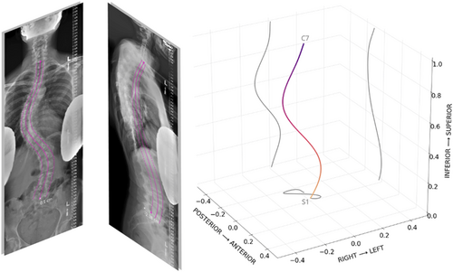
Per view, points along each side of the spine were fit using an polynomial degree 8, following an approach similar to the one proposed by Bonnani et al.26 Automatic quality control (autoQC) consisted of two tests: (1) polynomial fitting errors are below a predefined threshold and (2) predicted landmark order follows anatomical sequence, for example, L3 vertebrae landmarks should be positioned above L5 landmarks. The polynomial fitting threshold was set to 0.01, which was selected empirically by examining 100 predictions and identifying a cutoff with specific to low-quality predictions. The autoQC step was included as a safeguard to detect predictions from out of distribution inputs. Finally, per view, the vertebral midline curve was extracted by averaging points from each side and fitting a polynomial through the vertebra midpoints. Midlines and contours were overlaid onto input images for visualization. For 3D reconstruction, the S1 midpoint was defined as the origin and 0–1 normalization of the z-axis was used to scale the S1 to C7 distance between views, resolving slight differences in magnification. Coronal and sagittal midlines were each sampled with 1000 points, combined using a common z-axis, and isotropically normalized. Due to the lack of calibration objects in the field of view, three major assumptions were used to accomplish the reconstruction: patient posture did not change between acquisitions, intrinsic parameters of the x-ray source were identical for both acquisitions, and acquisition planes were orthogonal to one another. Plots with sagittal, coronal, and axial projections were used to visualize the resulting 3D curve (Figure 1).
2.4 Institution-wide validation
To further test algorithm validity and generalizability, predicted imbalance measurements were compared to measurements mined from radiology reports. Radiology reports were parsed with a simple regular expression tool to extract imbalance measurements in centimeters. Predicted results were visualized as scatterplots and error histograms, agreement was assessed using MAD and CCC. A final qualitative check of algorithm generalizability was performed by running inference on images from the 2019 Accurate Automated Spinal Curve Estimation (AASCE) challenge test set27 and examining the vertebral overlays.
2.5 Offline institution-wide inference
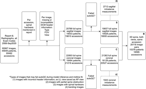
Musculoskeletal radiologists and neuroradiologists compiled an exhaustive list of 28 radiology exam codes to identify relevant patient accessions between 2008 and September of 2020. All associated Dicom images and reports were anonymized. Data filtering steps are detailed in a flowchart (Figure 2). First, accessions with radiology reports mentioning (“hardware,” “fusion,” “rods,” “screws”) were removed. Then, Dicom headers missing view or pixel information were excluded. The remaining 20,788 sagittal and 22,893 coronal images were preprocessed identically to the model development images, then run through the landmark detection and midline curve extraction algorithm. Approximately 6.6% coronal images and 4.5% sagittal images failed autoQC; failed images were primarily mislabeled views, patients with spinal hardware not mentioned in the report, and bending radiographs.
2.6 Shape modeling
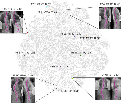
A total of 20,118 3D spines described by 2000 anatomically corresponding points were used to construct a statistical shape model. Features were centered before using Singular Value Decomposition based Principal Component Analysis to project the data to a lower dimensional, linear subspace. This resulted in 8 new shape axes (modes) describing shape variability within the patient population. In other words, the curvature of each 3D spine is described by 8 numbers, each describing specific shape characteristics. The average spine shape is visualized alongside −3 to 3 SDs of each shape mode to interpret shape characteristics. T-distributed stochastic neighborhood embedding (t-SNE) was used to visualize the distribution of patient spine shapes by creating a nonlinear embedding of the 8 dimensional shape vector into a two dimensional subspace. Twelve patients with scoliosis were randomly selected for Cobb angle evaluation: measurements from two trainees and one radiologist were averaged (R1, R2, radiology report) and plotted alongside the t-SNE datapoints.
2.7 Hosted model
For interested readers, the spinal landmark algorithm and radiology report parser is hosted on https://iriondo.github.io/. Anonymized lateral and frontal (AP) Dicom image pairs are required to extract spine contours, a 3D spine plot and shape parameters.
3 RESULTS
Dataset information for model development and institution-wide deployment is detailed in Table 1. From 2008 to early 2020, acquisition of spine radiographs has been growing at 19% per year. As a result, imaging acquired within the last 6 years constitutes a large proportion of the data used in this study. Ratio of female/male patients was consistent across all datasets (54.9%–66.2%) except Srad and Crad which were 87.5% and 83.3% female. Age distribution was bimodal, with a mean age of 12.6 (3.6) years for pediatric acquisitions and 58 (16) years for adult acquisitions.
| Dataset description and shorthand | Number of patients | Number of accessions | Number of images | Acquisition year | Patient age | Patient sex |
|---|---|---|---|---|---|---|
| Coronal full spine radiographs with curve prediction (C) | 16,129 | 20,527 | 21,382 | 2015 (2008, 2020) | 46.9 (1.16, 99.0) | 60.9% F |
| Sagittal full spine radiographs with curve prediction (S) | 15,628 | 19,000 | 19,857 | 2015 (2008, 2020) | 49.7 (0.59, 105.0) | 57.3% F |
| Radiographs with cm of coronal imbalance in report (iC) | 1450 | 1643 | 1643 | 2013 (2008, 2020) | 50.8 (4.0, 95.0) | 66.2% F |
| Radiographs with cm of sagittal imbalance in report (iS) | 2415 | 2712 | 2712 | 2013 (2008, 2020) | 55.3 (4.0, 95.0) | 60.7% F |
| Bi-planar full spine radiographs with 3D curves (B) | 15,378 | 18,595 | 20,118 | 2015 (2008, 2020) | 49.5 (1.16, 99.0) | 58.5% F |
| Radiographs measured for sagittal imbalance (Srad) | 8 | 8 | 8 | 2012 (2009, 2014) | 53.4 (20.0, 75.0) | 87.5% F |
| Radiographs measured for coronal imbalance (Crad) | 12 | 12 | 12 | 2011 (2009, 2014) | 51.8 (19.0, 75.0) | 83.3% F |
| Coronal radiographs with keypoint annotations (Calgo) | 188 | 194 | 194 | 2014 (2009, 2018) | 51.6 (4.0, 85.0) | 56.6% F |
| Sagittal radiographs with keypoint annotations (Salgo) | 366 | 366 | 366 | 2014 (2009, 2018) | 55.1 (4.0, 88.0) | 54.9% F |
- Note: Acquisition year and age are expressed as mean (range). Calgo, Salgo, Crad, and Srad were used for model development and validation; C, S, iC, iS, and B were used for institution-wide model deployment and validation. When the number of patients was less than the number of accessions for a given dataset, this indicated a subset of patients had more than one visit. When the number of images was greater than the number of accessions, a subset of patients had repeat images within the same accession.
3.1 Model testing
The spinal landmark detection models showed robust performance across the test set (Table 2). On average, pointwise MAE for coronal and sagittal images was <10 mm, with a majority of pointwise errors <5 mm and few errors >20 mm. The largest errors were driven by a shift in the superior-inferior axis, where predicted landmarks were placed on vertebra edges rather than corners due to regions with low image quality or disagreement on the location of the landmark endplates. Superior-inferior shift was preferable over anterior-posterior/medial-lateral shift since the former still allowed for accurate fitting of spinal contours. Although a direct comparison is not possible due to different training and testing datasets, transforming our landmark predictions and ground truth points to match Multi-View Correlation Network MVC-Net's19 scale we saw 79%, 66% lower test error (0.0095 vs. 0.0459, 0.0136 vs. 0.0398) in sagittal and coronal views, despite MVC-Net requiring both views as input.
| Number of images | Pointwise mean absolute error (mm) | Imbalance measurements (mm) | Imbalance mean absolute difference (mm) | Imbalance CCC | |
|---|---|---|---|---|---|
| Coronal radiographs with keypoint annotations, test (Calgo) | 28 | 8.68 CI (6.59, 11.0); range (3.6, 24.8) | 7.72 CI (2.32, 13.3); range (−19.6, 43.4) | 2.42 CI (1.57, 3.35); range (0.013, 10.3) | 0.973 CI (0.939, 0.989) |
| Sagittal radiographs with keypoint annotations, test (Salgo) | 40 | 5.44 CI (4.24, 6.87); range (1.97, 20.8) | 19.4 CI (6.65, 32.2); range (−62.3, 127.0) | 3.58 CI (2.59, 4.74); range (0.039, 14.3) | 0.993 CI (0.985, 0.997) |
- Note: “Imbalance measurements” column describes the distribution of the imbalance measurements defined by the ground truth landmarks.
- Abbreviations: Calgo, coronal algorithm; CCC, concordance correlation coefficient; CI, confidence interval; MAD, mean absolute difference; MAE, mean absolute error; mm, millimeters; Salgo, sagittal algorithm.
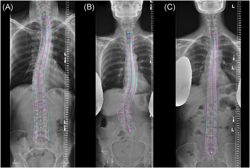
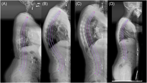
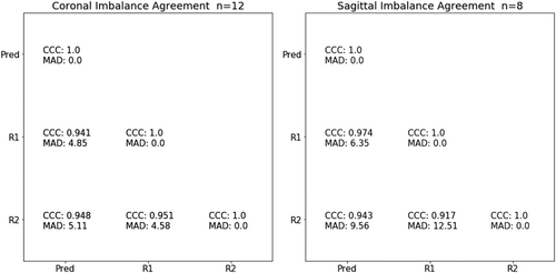
Overall, S1 and C7 endplate landmark identification and midline curve extraction was highly reliable, example overlays in Figures 3 and 4. Imbalance measurements derived from ground truth landmarks in the test set spanned from −19.6 to 43.4 mm of coronal imbalance and −62.3 to 127 mm of sagittal imbalance, and included patients with varied spinal deformities (Bland-Altman plots in Figure S2). Predicted imbalance measurements were in excellent agreement with landmark measurements (CCC of 0.993 and 0.973 for sagittal and coronal imbalance, respectively). In a small clinical dataset (Srad, Crad), algorithm imbalance measurements remained in good agreement with each radiologist: CCC of 0.974, 0.943 for sagittal and 0.941, 0.948 for coronal, MAD <10 mm for all samples (Figure 5). For sagittal imbalance rater-algorithm agreement was 3.3%–6.2% higher than inter-rater agreement. For coronal imbalance, rater-algorithm agreement was 0.3%–1.1% lower than inter-rater agreement.
3.2 Institution-wide validation
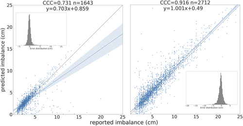
There was moderate agreement between radiology reports and predicted imbalance (CCC 0.916 sagittal, 0.731 coronal) (Figure 6 and Figure S3). Lower agreement in this dataset compared to the manually annotated dataset was expected given human errors in radiology reports and errors in automatic text parsing for label extraction. Differences >5 cm between reported measurement and predicted measurement were investigated: 60% caused by errors in reporting (e.g., sagittal and coronal measurements flipped, or use of qualifiers “more than”, “at least”), 18% from errors in text extraction (e.g., previous value for imbalance extracted from report), and 12% had report text and accession number potentially mismatched (deep learning prediction overlays are accurate but discordant with the reported measurements). This further demonstrated algorithm validity and generalizability to the institution-wide dataset, as this dataset included measurements from several radiologists and x-ray sources. Anatomically feasible predictions on the AASCE challenge images (Figure S4) suggested the landmark detection algorithm may be robust to shifts in patient population, data acquisition between institutions, and image compression.
3.3 Global alignment parameters
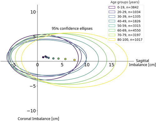
Sagittal and coronal imbalance were measured using predicted keypoints and image header information. Figure 7 shows the resulting mean value and 95% confidence ellipsoid of sagittal and coronal imbalance parameters by age group. After age 50, global sagittal alignment became increasingly positive.
3.4 Shape modes
A total of 8 shape modes (Figure 8) described 99.68% of shape variation in the patient population. Plotting curves at −3 to 3 SDs of each mode revealed several shape characteristics. Modes 1/3/7 were dominated by sagittal plane variations, while variations in Modes 2/4/8 were localized to the coronal plane. Modes 5/6 were a combination. Modes 1/2 accounted for 58.3%, 20.2% of the total shape variation and reflected changes in sagittal and coronal imbalance, respectively. Mode directions agreed with imbalance conventions (positive, negative). Mode 3 curves (11.5% of variation) had a single point of intersection near T6, where increasingly negative values showed exaggerated lumbar lordosis and posterior sagittal balance while positive values a C-shaped lateral spine and anterior sagittal balance. In the coronal plane, negative values were linked to a minor rightward thoracic curve.
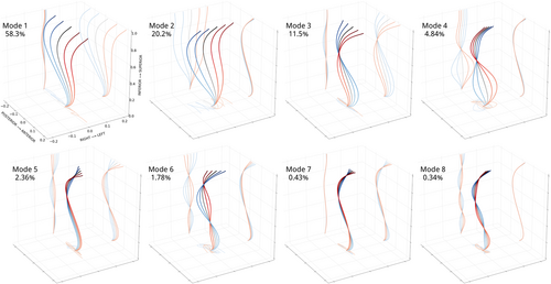
Mode 4 curves (4.84% of variation) had a single point of intersection near T11, negative values indicated major rightward lumbar curves, positive values major leftward curves, with curve magnitude scaling with mode values and a compensatory change in imbalance.
Mode 5 (2.36% of variation) and Mode 6 (1.78% of variation) curves had 2 points of intersection, near T4 and L2. Negative values of Mode 5 were linked to a “flat back” shape with a small rightward lumbothoracic curve, while positive values were associated with mid-thoracic kyphosis. Negative values of Mode 6 showed a double curve shape with a major rightward lumbothoracic curve and minor leftward lumbar curves and upper thoracic curves, with the opposite true for positive values. Last, Mode 7 (0.43%) and mode 8 (0.34%) plots had three intersection points and reflected local changes in sagittal and coronal curves. Positive values for Mode 7 were linked to upper thoracic kyphosis. While shape modes were interpreted using common clinical terms for spinal deformity, important observations were gleaned by examining shape mode plots. For example, positive and negative values in Mode 2 appeared mostly symmetric, however axial projections revealed a twisted loop shape in the negative values. Several axial projection shapes (further described in Pasha et al.28)—V-shape, S-shape, closed loop—were identified in this study. T-SNE embedding did not separate patients into visually distinct subgroups, and instead resulted in a large point cloud where the main directions of variation corresponded to variations in shape Modes 1 and 2. Patients with similar Cobb angle measurements were only colocalized if sagittal plane curves were also similar (Figure 9). Coloring the point cloud by age, sex, image acquisition year did not uncover any obvious patient clusters.
4 DISCUSSION
The developed landmark extraction algorithms demonstrated robust performance across the tested datasets. Once validated, algorithms were run on institution-wide data with pairs of frontal (anterior-posterior/posterior-anterior) and lateral (left-lateral) view radiographs to reconstruct approximations of 3D spine shape. A detailed discussion of merits and limitations of this approach is warranted.
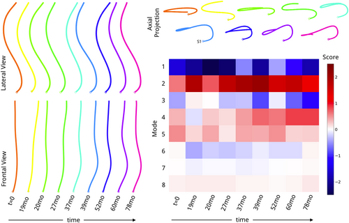
As a first point of merit, the proposed method could enhance current clinical assessment of spine radiographs. Landmark annotations are not feasible within the clinical workflow as they require significant user input and are vulnerable to user error. Several factors can reduce visibility and prevent the reliable manual identification of landmarks including severe spinal deformity, overlapping soft tissues, and visible lead shields. Moreover, anatomical landmarks may present differently in patients with obesity, osteoporosis, transitional anatomy, fused bone, or at variable skeletal maturities. The sacral plateau (S1) and lower endplate of C7 were chosen as reliable anchor points, since nearby anatomical landmarks (ribcage, spinous processes, sacrum) allow for reliable identification even in low visibility settings. Automatic imbalance measurements were validated using both manual annotations and a large clinical dataset, providing evidence of the accurate identification of these anchor points. The landmark prediction, midline curve fit, quality control, and 3D reconstruction for the proposed method are fully automatic and therefore have the potential to scale and integrate into the clinical workflow. Once deployed, prediction algorithms could run online—where clinicians would request results for a specific image pair—or offline—where inference would run on images shortly after acquisition and results would be stored in PACS. Due to lack of repeatability data, the proposed method could not be validated for the assessment of longitudinal changes in 2D and 3D spine shape (e.g., longitudinal case presented in Figure 10). Nonetheless, clinicians can be presented with a set of similar cases at their institution based on age, sex, and curvature similarity (defined as Mahalanobis distance in shape space, Figure 11). Retrieval of similar cases, as first proposed for coronal radiographs by Menon et al.,29 would allow for treatment planning based previous experiences with similar patients. Furthermore, similarity grouping would enable the identification of patient subgroups for retrospective observational research or provide prevalence estimates of specific spine deformities for future cohort designs.
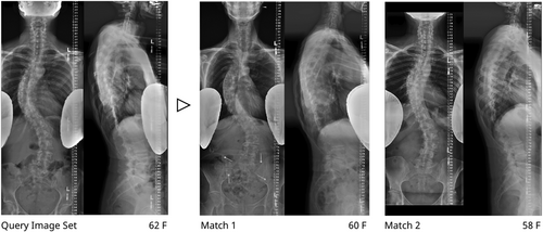
Second, an approximate 3D spine shape provides a rich description of global deformity compared to single plane evaluations, even with noise arising from an imperfect biplanar reconstruction. Shape mode embedding highlighted differences between patients with high curve similarity in the coronal plane but low similarity in the sagittal plane. Global curvature informs the distribution of biomechanical loads on the spine and might be important to understand risk of curve progression and assist in clinical management.30 For example, recent AIS literature showed that preoperative 3D shape, early postoperative shape, and information on fusion levels could be used to predict surgical outcomes 2 years post-op.28 A significant body of literature exists on classification of 2D and 3D spine shapes for AIS and ASD patients.1, 31 While it would be worthwhile to see if these classes naturally group in 3D shape space, the proposed method does not impose a specific classification scheme on the results, thereby more appropriately displaying the spectrum of spinal deformities and providing a common basis to compare different patient populations.
Third, it is well known that deep learning models are sensitive to shifts in data acquisition and can behave unexpectedly when tested on new populations.32 Understanding how performance is affected by severe domain shift will require additional investigation. Therefore, we have hosted the algorithms online such that they are easily accessed by the research community. To our knowledge, we are the first testable algorithm for spine midline extraction from biplanar radiographs, with an approximate runtime of 20 s per image pair (Figures S5–S6).
A major limitation of the proposed method is that the 3D curve reconstruction is only an approximation of 3D shape since it is based on two noncalibrated acquisition planes. Calibration of the two image planes was not feasible for this study as the minimum set of parameters required to establish stereocorrespondence using epipolar geometry (six anatomical landmarks per vertebra, known calibration parameters, a known distance landmark for scale or focal length information) were not available on all images. Additionally, published methods that perform self-calibration on landmarks such as spinal contours or midlines rely on statistical shape models based on separate databases of computed tomography scans to infer or constrain a full 3D spine reconstruction.33-35 Given our interest in understanding global shape variations across our institution we opted against using pre-existing shape models for reconstruction as these would not capture the wide variety of spine shapes in our dataset. It is important to emphasize that limitations associated with noncalibrated acquisitions apply to all spine measurements performed on biplanar radiographs including imbalance, Cobb angles, lordosis, kyphosis, and pelvic parameters. If the orthogonality assumption is not met between frontal and lateral views, it is possible the maximum curvature would be underestimated. It follows that our proposed method would not be appropriate for applications where high-precision 3D skeletal reconstructions of pedicles and vertebral bodies are required, such as patient-specific computational models.
Calibration and issues with patient movement can be addressed during acquisition by using dedicated simultaneous low-dose stereoradiographic (EOS) systems achieving equivalent or improved image quality and measurement reliability with less radiation than a conventional radiograph.36, 37 While this technology holds great promise, upgrading to these systems can be cost-prohibitive. In addition, even institutions with EOS systems can benefit because they have a wealth of data before EOS that could be analyzed retrospectively and used to aid clinical decision making.
A minor limitation of the proposed method is the limited scope of the development dataset. While the dataset included a wide range of spinal deformities (similar to pathological ranges reported in the literature9, 38), radiograph sources, and demographics, it did not include bending or postoperative radiographs. Therefore, an abstention mechanism was built into the pipeline: algorithm predictions for these out-of-distribution images have high variability and are flagged as invalid during the autoQC step. Automatic landmark prediction for instrumented spinal radiographs has been investigated in,20 but was considered out of the scope for this study given that key landmarks are often obscured.39 Furthermore, fused spinal levels in an instrumented patient population were likely to result in different spine shape modes as compared to the pre- or nonoperative population. Moreover, shape mode results should be interpreted with caution due to sampling bias: the patient population undergoing full spine X-rays are not likely a representative sample of the general population.
The most surprising finding in this work was the range in actual sagittal and coronal imbalance among images linked to radiology reports stating “no imbalance.” We ran inference on images whose radiology reports stated “no imbalance” and found true measurements of approximately ±2.5 cm of coronal imbalance and ±5 cm sagittal imbalance (Figure S3). This has important implications: when no exact measurement was provided, qualitative descriptions of spinal alignment (“no imbalance,” “neutral balance,” “mild”) were subjective.
Future work will focus on: (1) Testing and documenting the landmark algorithms’ robustness to domain shift and identifying new failure modes. Specifically, automatic vertebral midline extraction and shape modeling will be tested on radiographs pooled from several collaborating institutions. Moreover, individual researchers are encouraged to test the algorithm online and provide feedback, reporting cases of success or failure. This follows guidelines outlined in a recent review of machine learning for scoliosis by Chen et al.40 calling for “heterogenous test sets” for spine deformity research and evaluation of ML tools by multidisciplinary teams. (2) Using a curated subset of preoperative AIS, ASD images and surgical outcomes, determining if specific partitions of the 3D shape space may have more favorable surgical response.
In summary, this study describes a new method for automatic extraction of the vertebral midline from biplanar radiographs and a method describing 3D spine shapes through 8 interpretable shape modes. Deployed institution-wide, this method has the potential to enhance clinical assessment of spine deformities.
ACKNOWLEDGMENTS
The Back Pain Consortium (BACPAC) Research Program is administered by the National Institute of Arthritis and Musculoskeletal and Skin Diseases (NIAMS). This research was supported by the National Institutes of Health through the NIH HEAL Initiative under award number UH2AR076724-01. The content is solely the responsibility of the authors and does not necessarily represent the official views of the National Institutes of Health or its NIH HEAL Initiative.
The authors would like to acknowledge Gaurav Inamdar and Carla Kinnunen for assistance with image annotation.
AUTHOR CONTRIBUTIONS
Claudia Iriondo: research design, algorithm development, experiment analysis, and manuscript drafting. Sharmila Majumdar: Algorithm development. Rutwik Shah, Upasana Bharadwaj, and Emma Bahroos: data curation and annotation. Cynthia Chin and Mohammad Diab: research design and critical revision of the manuscript. Valentina Pedoia and Sharmila Majumdar: obtaining funding, research design, experiment analysis, and critical revision of the manuscript. All authors read and approved the final manuscript.


