Dynamics of worker flows and vacancies: evidence from the sign restriction approach
Abstract
This paper establishes robust dynamic features of the worker reallocation process in the US labor market. I use structural VARs with sign restrictions, which take the form of restricting the short-run negative relationship between vacancies and unemployment (i.e., Beveridge curve). Despite the ‘weakness’ of these restrictions, they reveal a clear, unambiguous pattern that, when unemployment increases and vacancies drop, (i) both the separation rate and gross separations rise quickly and remain persistently high, (ii) the job finding rate and vacancies drop in a hump-shaped manner, and (iii) gross hires respond little initially, but eventually rise. These results point to the importance of job loss in understanding US labor market dynamics. This pattern also holds with respect to different kinds of shocks that induce the same Beveridge curve relationship. This paper also considers the ‘disaggregate model’, which uses data disaggregated into six demographic groups and incorporates transitions into and out of the labor force. I show that the separation rate continues to play a dominant role among prime-age male workers, while, for other groups, changes in the job finding rate are more important. Copyright © 2009 John Wiley & Sons, Ltd.
1. INTRODUCTION
The purpose of this paper is to provide robust dynamic features of the worker reallocation process in the US labor market. In particular, I pay close attention to the variables useful for evaluating the quantitative abilities of the Mortensen–Pissarides search/matching models that are widely used in macro/labor economics. There have been a number of recent papers that examine empirical regularities of job separation and finding rates, the key variables driving unemployment fluctuations in these models. Recent papers by Hall (2005a,b) and Shimer (2007) argue that the separation rate into unemployment is acyclical in the data. This claim has led many researchers in the field to write down models that assume that separations of workers from their employers occur at a constant rate, regardless of the aggregate conditions.1 In essence, those papers attempt to account for unemployment fluctuations from variations in the job finding rate alone. A number of subsequent papers, however, have challenged the Hall–Shimer view, arguing that the separation rate is countercyclical (e.g., Elsby et al., 2009; Fujita and Ramey, 2006, 2009; Fujita et al., 2007; Yashiv, 2007). The implication is that it is important to model the separation margin as well as the hiring margin to fully understand unemployment dynamics.
The papers referenced above, however, rely mostly on descriptive measures for their evaluations of the data. This can potentially be problematic because those measures may be influenced by variations of the data that are not relevant to evaluating the search/matching models, in which variations of the data are driven entirely by the exogenous structural shocks, such as the productivity shock. This paper instead attempts to characterize empirical regularities of the observed data conditional on the structural shock relevant for the evaluations of this class of models. I identify the structural shock by using VAR models in which the data generating process of the separation rate, the job finding rate, and vacancies is explicitly specified. Given the dynamic paths of these three variables, I further trace the paths of gross separations and hires, and thereby the stock of unemployment.
In identifying the structural shock, I make use of the sign restriction approach developed by Uhlig (2005) and others.2 This approach is useful for my purpose because it identifies the shock by imposing only minimal sign restrictions on the pattern of impulse response functions and considers all possible responses consistent with those restrictions. Specifically, I identify the ‘aggregate shock’ by imposing restrictions on the signs of responses of unemployment and vacancies (i.e., the Beveridge curve relationship). I assume that in response to the negative shock unemployment rises for at least a few quarters, while vacancies drop in the impact period. I argue that these restrictions are consistent with a wide range of Mortensen–Pissarides style search/matching models with and without the endogenous job separation decision. A nice feature of this approach is that the shock is identified without imposing any restrictions on the behavior of the transition rates, making it possible to assess how they respond to the identified shock. Furthermore, as mentioned above, the approach allows me to trace not only the behavior of transition rates but also the behavior of gross worker flows in one unified framework. I argue that it is important to consider gross flows as well as transition rates, because it greatly helps distinguish the implications of the matching models with and without endogenous separation.
Recent papers by Paustian (2007) and Fry and Pagan (2007), however, cast doubt on the usefulness of the sign restriction approach. They show in other applications of the sign restriction approach that the method often yields ambiguous results, especially when the restrictions are weak, and thus the approach is simply uninformative for the question under investigation. In my application, however, the identification produces the following unambiguous features of the US labor market. When the negative aggregate shock occurs, (i) both the separation rate and separation flows rise quickly and remain persistently high in the subsequent periods, (ii) the job finding rate and vacancies drop in a gradual and hump-shaped manner, and (iii) gross hires respond little initially, but eventually rise in later periods. These results can be considered robust given that these features emerge even under such weak restrictions. Findings (i) and (ii) indicate that fluctuations in both the separation and the job finding rate play an important role in shaping unemployment fluctuations over the business cycle. The third finding, which says that gross hires move in a countercyclical manner, suggests that the separation rate plays a dominant role in understanding gross hires as well as gross separations. To illustrate the mechanism behind this pattern, I compute the contribution of each transition rate for unemployment fluctuations by fixing either the separation rate or job finding rate at the steady state level and examining the hypothetical paths of the remaining variables. When the separation rate follows estimated paths while the job finding rate is held fixed, unemployment increases because of the higher separation rate and hence more separation flows. Because job finding takes place at the same fixed rate, the increases in unemployment result in more hires, which is consistent with the actual paths. On the other hand, when the separation rate is fixed while letting the job finding rate follow the actual estimated paths, gross hires go down, not up, because of the direct consequence of slower job finding. Although only illustrative, it indicates that ignoring fluctuations in the separation rate paints a misleading picture of US labor market dynamics.
Several recent papers also use structural VARs to assess the labor market responses to different types of structural shocks, such as technology shocks and demand shocks (e.g., Braun et al., 2007; Canova et al., 2007). My benchmark VAR is obviously silent about the effects of these different types of shocks. Therefore, the question is: Do those different shocks produce different worker reallocation patterns and, if so, how different?3 I therefore expand the benchmark model by adding the inflation rate and productivity growth. By applying the sign restriction approach to the expanded model, I identify the demand and technology shocks. For the identification of the demand shock, I restrict the price behavior together with the behavior of the labor market variables. A similar idea has been used in the literature (e.g., Peersman, 2005; Braun et al., 2007). The technology shock is identified by imposing a sign restriction on the long-run behavior of labor productivity as in Dedola and Neri (2007). Combining this long-run sign restriction on labor productivity with the basic implication of the Schumpeterian vintage model, put forth by Michelacci and Lopez-Salido (2007) and Canova et al. (2007), allows me to consider the effects of the technology shock.4 The results show that these two kinds of shocks yield qualitatively the same pattern of labor market adjustments, meaning that higher unemployment is associated with the higher separation rate and lower job finding rate. In other words, labor market reallocation takes place in a similar manner regardless of the nature of the shocks and that the worker reallocation pattern summarized by the benchmark trivariate VAR is quite robust.
The first clear message from the findings in this paper is that the models with exogenous separation miss an important part of the story behind unemployment dynamics, as opposed to the view put forth by Hall (2005a,b) and Shimer (2007). In my view, future research would thrive around the models with endogenous separation decisions such as those of Mortensen and Pissarides (1994), Den Haan et al. (2000) and Ramey and Watson (1997). Another robust finding of this paper is that the responses of vacancies and the job finding rate always exhibit a hump-shaped pattern. In Fujita and Ramey (2007), we show that the standard matching model with and without endogenous separation fails to capture the delayed and persistent responses. This finding suggests that enriching the job creation side of the model is also an important avenue for future research.
The main part of the paper summarized so far focuses on labor market transitions between employment and unemployment, ignoring the out-of-the-labor-force state, as is often the case in the literature. In Fujita and Ramey (2006), however, we point out the presence of an important heterogeneity across different demographic groups in the pattern of worker reallocation, which emerges when transitions into and out of the labor force are explicitly taken into consideration. I therefore also consider the ‘disaggregate model’, where a VAR is formulated with the transition rates for six demographic groups together with the aggregate vacancy series. This system allows me to trace both disaggregate- and aggregate-level behavior of gross flows and the stock of unemployment. The aggregate shock is again identified by restricting aggregate-level unemployment and vacancy behavior. I show that the pattern of worker reallocation found in the aggregate model continues to hold among prime-age male workers, thus suggesting an important role of separation. Among other groups of workers, on the other hand, countercyclicality of the separation rate becomes unclear, while the job finding rate continues to respond procyclically, which indicates dominance of the hiring activity. These findings point to the importance of explicitly considering heterogeneity across demographic groups and the participation decision in modeling labor market reallocation over the business cycle.
This paper proceeds as follows. Section 2 reviews the sign restriction approach in a general setting. In Section 3, I apply the method to the labor market data. I first present the benchmark results based on a small VAR with only the labor market variables. The expanded model is then estimated to show the robustness of the labor market responses with respect to the different types of shocks. Section 4 extends the aggregate model to a larger disaggregate model that includes the data for the six demographic groups. Section 5 concludes the paper by discussing the implications for quantitative macro/labor literature.
2. REVIEW OF THE METHOD
 (1)
(1) (2)
(2) . Let ωt be an n × 1 vector containing time-t values of structural disturbances. The reduced-form residuals and structural disturbances are linked through
 (3)
(3) (4)
(4) (5)
(5)With an estimate of Σ at hand, the identification problem amounts to uncovering the  free elements in A by imposing identifying restrictions.
 (6)
(6) (7)
(7)Computations
For each set of the estimates for (Φ, Σ), we can compute impulse vectors and hence impulse response functions corresponding to different unit vectors in an n-dimensional sphere. To uniformly cover the points on the n-dimensional space, I make use of the following algorithm: I generate n numbers from a normal distribution with mean zero and standard deviation one, treat them as coordinates, and normalize the resulting vector into a unit vector. The normalized n-dimensional vector corresponds to each point on the sphere. We can repeatedly generate n-dimensional vectors to uniformly cover the sphere.5
I deal with the sampling uncertainty about the VAR parameters (Φ, Σ) in a Bayesian manner. As in Uhlig, I assume that prior and posterior distributions for (Φ, Σ) belong to the Normal-Wishart family. Let  and
and  be the MLE for Φ and Σ, respectively. Under the use of a non-informative prior, the Normal-Wishart posterior distribution is characterized by (i) Σ−1 follows a Wishart distribution
  with E[Σ−1], where T is the sample size, and (ii) conditional on Σ, the coefficient matrix Φ in its column-wise vectorized form, vec(Φ) follows a multivariate Normal distribution
  , Σ⊗(X′X)−1), where X = [Y1, …, YT] with Xt = [Y′t−1, …Y′t−m]. I use the Matlab routines wishrnd and mvnrnd to simulate the Normal-Wishart posterior distribution.
I simulate 1000 pairs of Σ and Φ. For each pair, I evaluate 1000 unit vectors on the n-dimensional sphere. Thus a total of 1,000,000 q's and impulse vectors are evaluated. After computing each set of the impulse response functions corresponding to each unit vector, I check if the sign restrictions are satisfied. I store only the impulse vectors that meet the restrictions.
3. APPLICATIONS TO US LABOR MARKET DYNAMICS
This section applies the sign restriction approach explained above to US labor market data. The benchmark model specifies a VAR model with three variables: the separation rate, the job finding rate, and vacancies.6 This system includes the vacancy series, capturing firms' recruitment efforts as in the search/matching models.
The benchmark identification relies on the restrictions on the behavior of unemployment and vacancies (i.e., the Beveridge curve relationship). Because of the parsimonious nature of the identifying restrictions, this VAR is unable to separate out those shocks that induce the same qualitative patterns in the unemployment and vacancy responses. Later in this section, I estimate the expanded model that includes more variables (i.e., the inflation rate and labor productivity growth) in the VAR, which allows me to identify those underlying shocks.
3.1. Data
Transition rates
I adopt two transition rate series from my previous paper (Fujita and Ramey, 2006). The series are available at monthly frequency, but I use the quarterly averages of the monthly data, since the productivity series, which I will use later in the expanded model, is available only at quarterly frequency. The sample period spans 1976Q1 through 2005Q4. Fujita and Ramey (2006) correct for so-called margin error in the CPS, building on the method developed by Abowd and Zellner (1985). The margin error refers to inconsistency in the stock-flow identities. In the CPS, labor market transition information can be computed for at most 75% of all the individuals included in the stock calculations. If the information is missing at random, the missing observations per se should not cause important inconsistencies, given that the sample size is large.7 However, it is known that the missing individuals, amounting to at least 25% of the sample size, create systematic biases in the flow calculations. Fujita and Ramey therefore parameterize true flows as flexible nonlinear functions of the missing-at-random flows and minimize the distance between the stocks implied by the parameterized flows and the official CPS stocks by the use of nonlinear regressions. Our model nests the missing-at-random model, and the data strongly reject the latter model.8
 (8)
(8) (9)
(9) and p̂t are the average separation rate and average job finding rate, respectively, measured by the CPS's discrete-time observations at time t, and where variables without hats are corresponding hazard rates. Given that I focus on transitions between the two states, employment and unemployment, average transition rates are computed as

Treatment of NILF flows
It is well known that there are large flows into and out of the not-in-the-labor-force (NILF) state (e.g., Abowd and Zellner, 1985; Blanchard and Diamond, 1989). In Fujita and Ramey (2006), we propose a sensible way of incorporating such flows into the two-state framework above; however, they show that when the NILF flows are incorporated, the aggregate behavior of the transition rates and flows paints misleading pictures of US labor market dynamics. In particular, they show that breaking down the aggregate data into demographic groups reveals important differences in the cyclical behavior of young workers and prime-age workers. In Section 4 I incorporate NILF flows into the analysis, while in this section I focus on transitions between employment and unemployment, as is often the case in the literature.9
Vacancies
I use the index of help-wanted advertisements released by the Conference Board as an approximation for vacancies. Because this series simply represents the index of the aggregate number of newspaper help-wanted advertisements in 51 major newspapers in the USA, the approximation may be crude. However, there are several pieces of evidence that this series closely tracks the cyclicality of actual job vacancies in the USA.10 The series is available at monthly frequency starting in January 1951, but I use the quarterly averages over 1976Q1 through 2005Q4.
Detrending
The first two panels of Figure 1 plot the seasonally adjusted data for the job finding rate pt and the separation rate λt. While the job finding rate does not seem to have noticeable trending behavior, the separation rate has been drifting down since the early 1980s.11 The last panel shows the vacancy series, which also appears to exhibit low-frequency movements. In particular, one can observe a significant downward trend in recent years, which can be attributed to a shift of recruitment methods from newspaper ads toward other methods such as the Internet. Note, however, that there is no a priori reason why such a shift of recruitment methods would affect the cyclicality of the data.
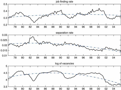
Data. Note: Transition rates are quarterly averages of the monthly series constructed by Fujita and Ramey (2006), and seasonally adjusted by Census X-12. The index of help-wanted advertisements represents the vacancy series. The seasonally adjusted series is released by the Conference Board. The trend components are identified by regressing on time polynomials of up to second order. This figure is available in colour online at wileyonlinelibrary.com/journal/jae
To remove such low-frequency movements from the analysis, I detrend the data by using deterministic quadratic trends. Taking a stand on how to detrend the data is necessary because the models of interest to me (i.e., search/matching models) do not exhibit such low-frequency trends. The trend components are also plotted in Figure 1, which shows that, as expected, the job finding rate has a flat trend, whereas the separation rate and vacancies exhibit trends that initially rise and then gradually decline over time. The trend of the last two variables is well captured by the quadratic trend. While I believe that the use of the quadratic trend reasonably takes out the low-frequency movements of the data that are outside my interest, there is an uncertainty regarding the specification of the trends. Later in this section, I check the robustness of the results with respect to alternative treatment of the trend.
Lag length
I use three criteria to choose the lag length: the Akaike information criterion (AIC), Schwarz criterion (SC), and Hannan–Quinn criterion (HQC). For the benchmark trivariate VAR described above, all three criteria suggest a lag length of two quarters. The main results below are therefore based on a lag length of two quarters. Again, later in this section, I look at the sensitivity of the results with respect to alternative lag length.
Tracing gross flows and unemployment
 (10)
(10) (11)
(11) , where
  and p̄ are historical averages.12 Note again that λt and pt are hazard rates in continuous time obtained based on the CPS's discrete time observations through equations (8) and (9), and that lt and ht therefore capture all flows that occur over the month under the assumption that hazard rates are constant over the period. See Appendix B of Fujita and Ramey (2006) for details. Fujita and Ramey further note that
 (12)
(12)The recent literature, such as Shimer (2007), Fujita and Ramey (2009) and Elsby et al. (2009), focuses exclusively on the behavior of transition rates without any reference to gross flows. The earlier literature, however, puts more emphasis on gross flows. For example, Blanchard and Diamond (1989, 1990) estimate the VAR with CPS worker flows constructed by Abowd and Zellner (1985) for answering questions similar to those in this paper. But they do not consider the behavior of transition rates. My approach above, which traces in a unified framework not only responses of transition rates but also gross flows and thereby the stock of unemployment, provides a more comprehensive look at labor market dynamics.13
3.2. Identification: Sign Restrictions
-
Restriction 1: The negative aggregate shock causes changes in unemployment to be non-negative for at least K quarters.
-
Restriction 2: The negative aggregate shock does not raise vacancies in the impact quarter.
In the benchmark specification, I set K to 2. But I examine the sensitivity of the results with respect to the value of K. These restrictions identify the shock that induces the movement along the Beveridge curve and are consistent with various specifications of the class of search/matching models.15 I use the term ‘aggregate shock’, meaning that it is supposed to capture the disturbance that equally hits the profitability of the employment relationships.
3.2.1. Relation to the Search/Matching Models
Textbook model with exogenous separation
First, consider the simplest possible form of the labor matching model (like those in Pissarides, 20 000, Ch. 1; Shimer, 2005; and Hagedorn and Manovskii, 2008) where the aggregate disturbance to the match productivity is the only shock to the economy and where the matches are dissolved at an exogenously specified rate. Other standard features of the model include linearity of the utility function, linearity of match production technology and no on-the-job search.16 In this model, the aggregate shock lowers the return from forming a match and therefore depresses vacancy postings and, as a consequence of lower hiring, the unemployment rate rises. Despite the bare-bones nature of this model, many researchers take very seriously the quantitative implications of the model. The two sign restrictions are clearly consistent with the implications of this model and therefore useful for evaluation of this class of model.
Extension to the RBC model
An extension of the model to the general equilibrium real business cycle model is considered by Merz (1995) and Andolfatto (1996). These papers maintain the single shock assumption (a shock to TFP of the representative match is the only shock in the model). Their results indicate that the key addition to the simpler model, the endogenous interest rate fluctuations, does not alter the vacancy–unemployment comovement imposed above. Again, a negative TFP shock lowers the return from forming a match and thus induces declines in vacancies and increases in unemployment.
Model with endogenous separation
Mortensen and Pissarides (1994) made an important breakthrough by endogenizing the separation decision.17 In the model, matched worker–firm pairs are subject to the idiosyncratic productivity shock as well as the aggregate shock. During the downturn, matches that have become less productive than cut-off productivities are destroyed. The cut-off productivities are higher during the downturn, thus generating the countercyclical separation rate. An important feature of the model is that the vacancy response is ambiguous: even though lower returns from forming a match discourage vacancy postings, the adverse shock causes the separation rate and thus unemployment to jump up, which encourages vacancy postings because the increased number of job seekers raises the job filling rate for firms. The second channel counters the first channel, thus making it a priori difficult to qualitatively predict the effect of the negative shock.18 Despite the theoretical ambiguity of the vacancy response, I chose to impose Restriction 2. From an empirical point of view, it seems far-fetched to argue against the second restriction on the basis of the theoretical ambiguity, given that the Beveridge curve relationship is accepted as one of the most robust empirical phenomena.19 The literature has proposed a couple of ways to make vacancies procyclical in the model. One of the ways is to introduce on-the-job-search into the model (e.g., Tasci, 2007; Ramey, 2008). This extension makes the vacancy behavior in the model more in line with the observed behavior.
Monetary DSGE model
Cooley and Quadrini (1999) is an earlier attempt to embed search/ matching into neoclassical monetary DSGE models. Both of these papers feature the endogenous separation decision. Their numerical results show that the money growth shock produces behavior of vacancies and unemployment consistent with the two restrictions imposed above. Walsh (2005) and Trigari (2009) consider the effects of the monetary policy shock in a new Keynesian framework with labor market matching and endogenous separation. Their results on the effects of the monetary policy shock are also consistent with my restrictions.20
3.2.2. Relation to the Older Literature
There is a branch of literature generated by Blanchard and Diamond's (1989) influential work. As in this paper, they identify the aggregate shock, assuming that the shock moves unemployment and vacancies in opposite directions.21 This assumption is challenged by several authors. In particular, Hosios (1994) develops a matching model where the unemployment–vacancy relationship is inconclusive about the nature of the shock. The subsequent literature avoids this problem by imposing sign restrictions on the pattern of worker turnover (e.g., transition rates, gross worker flows) instead of the unemployment–vacancy relationship. For example, Davis and Haltiwanger (1999) assume that the positive aggregate shock raises the job creation rate while it lowers the job destruction rate in the impact period. Balakrishnan and Michelacci (1999) use similar identifying restrictions on worker flows. In the context of this paper, similar restrictions can be imposed on the behavior of the separation and job finding rates (i.e., the positive aggregate shock is associated with the lower separation rate and higher job finding rate). Because unemployment necessarily decreases in this case, adopting this strategy amounts to dropping the assumption on vacancies. In my earlier paper (Fujita, 2004), I follow this strategy. While there are minor differences in the actual formulation of the underlying VAR and the data used, I show in that paper that the Beveridge curve relationship indeed emerges even without constraining the vacancy behavior at all. This suggests that the skepticism toward the Blanchard–Diamond strategy is not warranted, at least for the US data.
For the current paper, I experimented with the case in which the separation rate and the job finding rate were assumed to move in opposite directions in the impact period (with no restrictions on vacancies). I found that the resulting impulse responses from this alternative identification are very similar to the ones from the benchmark identification.22 This finding implies the robustness of the benchmark results along this dimension as well.
3.2.3. Are the Restrictions too Weak?
Although the two sign restrictions are consistent with the characteristics of the search/matching models in various forms, these restrictions do not allow me to disentangle the effects of different types of structural shocks that bring about the same qualitative Beveridge curve relationship. The benchmark results thus can be viewed as an average effect of the underlying shocks.
However, a potential problem of this approach is that these two restrictions are simply too weak to learn anything about the worker reallocation process. A recent paper by Paustian (2007) addresses the issue in different contexts.23 His main result is that sign restrictions are not useful for identifying the structural shock unless (i) the variance of the shock under inspection is large enough and (ii) the researcher imposes sufficiently numerous restrictions. By applying the sign restriction approach to the data generated from the model by Erceg et al. (2000), he shows that imposing only a small number of model-consistent sign restrictions does not pin down the response of output (i.e., output may fall or rise) even though the true output response is negative.24
Of course, whether or not sign restrictions are useful depends on the particular case under consideration. In the context of this paper, the implication of Paustian's criticism is that my sign restrictions are simply too weak to tell how worker flows respond to the identified shock. However, as will be seen in the following section, the two restrictions indeed uncover a very clear picture regarding the responses of worker transition rates, implying that Pustian's criticism does not apply in my case.
Apart from the inference issue regarding the identification through sign restrictions, it is also of economic interest to disentangle the effects of different underlying shocks. To this end, I consider the five-variable VAR, in which I distinguish between the demand shock and the technology shock.
3.3. Benchmark Results
Impulse response functions
Figure 2 displays responses of transition rates and worker flows. The impulse responses of changes in unemployment, the stock of unemployment and vacancies are separately plotted in Figure 3. The three lines in the figures represent the 16th, 50th and 84th percentiles of the simulated posterior distribution.
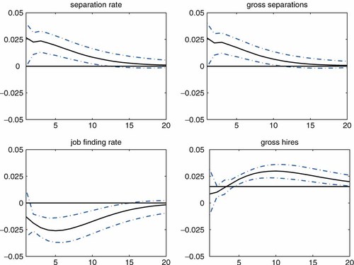
Impulse response functions for transition rates and worker flows. Notes: The shock is identified by imposing Restrictions 1 and 2. The black solid line represents the median of the posterior distribution. The error band represents the 16th and 84th percentiles of the posterior distribution. Responses are expressed as log deviations from the steady-state levels. This figure is available in colour online at wileyonlinelibrary.com/journal/jae
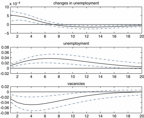
Impulse response functions for the change in unemployment, stock of unemployment and vacancies. Note: The shock is identified by imposing Restrictions 1 and 2. The black solid line represents the median of the posterior distribution. The error band represents the 16th and 84th percentiles of the posterior distribution. The response of changes in unemployment is expressed as a level deviation from the steady-state level (zero). Responses of the stock of unemployment and vacancies are expressed as log deviations from the steady-state levels. This figure is available in colour online at wileyonlinelibrary.com/journal/jae
The panels in the left column of Figure 2 show that the negative aggregate shock identified by the Beveridge curve relationship leads to increases in the separation rate and declines in the job finding rate. More specifically, observe first that even though the responses of the transition rates are not restricted at all, both series significantly deviate from their steady-state levels. The only case in which the sign of the response is ambiguous is the response of the job finding rate in the first quarter. Further, notice that (i) the separation rate quickly reaches its highest level, whereas the job finding rate follows a hump-shaped pattern, reaching its lowest level after about a year or so, and (ii) the largest deviations from their steady-state levels are of similar magnitude, suggesting that the two margins contribute roughly equally to unemployment fluctuations. Given the findings by Paustian (2007) discussed above, the fact that both transition rates respond strongly to the shock can be considered to be a robust characteristic of the US labor market, in contrast to the view put forth by Hall (2005a,b) and Shimer (2007) that unemployment dynamics are driven by fluctuations in the job finding rate alone.
The right column of Figure 2 presents responses of gross separations and hires. Not surprisingly, gross separations behave similarly to the separation rate because the pool size—the employment rate—is always close to one. The response of gross hires is not distinguishable from zero in the first few quarters. However, gross hires subsequently rise to a level higher than the steady-state level. This countercyclicality of hires may sound somewhat counterintuitive, given that the job finding rate is procyclical. Note, however, that the number of job seekers (unemployment) rises in the face of the adverse shock, and therefore it is a priori unclear whether the negative shock increases or decreases gross hires. The countercyclicality result thus suggests that the ‘pool size effect’ outweighs the effect from slower job finding.
One can see in the top panel of Figure 3 that changes in unemployment are restricted to being non-negative for the first two quarters. Accordingly, the stock of unemployment, plotted in the middle panel, keeps rising for the same period, generating hump-shaped responses. The last panel shows that the initial response of vacancies is restricted to being non-positive, but responses in the subsequent periods exhibit again the hump-shaped pattern. Note that, while I impose the restriction that the unemployment response be hump shaped, such restrictions are not imposed on the vacancy response. Combining the responses of unemployment and vacancies forms the familiar Beveridge curve relationship. As emphasized by Fujita (2004) and Fujita and Ramey (2007), the search/matching model in its standard form is unable to generate such hump-shaped patterns in vacancies.25
Plausibility of the sign restrictions
Although the above results clearly summarize the labor market dynamics in the USA, it is important to make sure that the identified shock accounts for significant portions of variations of the variables of interest. Figure 4 displays three panels showing the portion of the variances explained by the aggregate shock for each horizon. The results show that, although the error bands are quite wide as is often the case in this kind of exercise, the median estimates amount to around 40–50% for all variables.
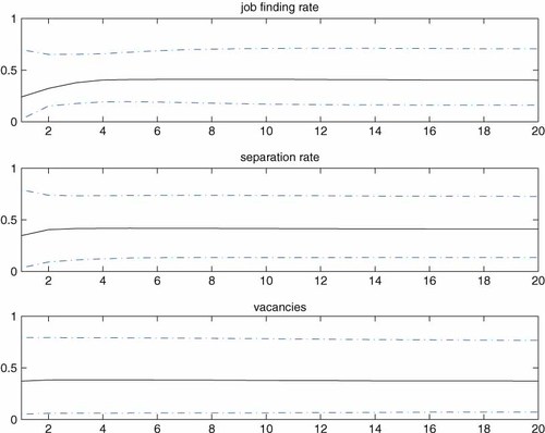
Variance decomposition. Note: The shock is identified by imposing Restrictions 1 and 2. The black solid line represents the median of the posterior distribution. The error band represents the 16th and 84th percentiles of the posterior distribution. This figure is available in colour online at wileyonlinelibrary.com/journal/jae
Another way to gauge the plausibility of the imposed sign restrictions is to calculate the fraction of the total draws that satisfy the restrictions. The acceptance rate amounts to 35%, confirming the plausibility.
Importance of separation rate vs. job finding rate
Recently, there has been a debate in the literature as to which margin—job finding rate or the separation rate—is more important in explaining unemployment fluctuations. The results above have already indicated that both margins are important. But to gain more insight into the quantitative importance of the two margins, I conduct the following simple exercise, in which either λt or pt is fixed at the steady-state level and examine the hypothetical paths of the remaining variables. Specifically, by plugging a constant path for either one of the two variables and the estimated path of the other into (10) and (11), the hypothetical paths for gross separations and hires, and thereby changes in unemployment and the stock of unemployment under each scenario, can be traced. I can then compare the hypothetical paths of these variables with the estimated responses.26
First, consider the case where the job finding rate is held fixed at the steady-state level. The results are shown in Figure 5. Note that even though the job finding rate is fixed, it is entirely possible that gross hires move considerably. This is because changes in the separation rate result in changes in the number of job seekers (the stock of unemployment) and therefore gross hires can move even under the fixed job finding rate. Further, the path of gross separations under this exercise is different from the actual estimated paths. However, the right top panel in the figure shows that gross separations behave very similarly to the estimated paths under the fixed rate of job finding. The second row presents the hypothetical path of the job finding rate (which is constant by construction) and gross hires. Somewhat surprisingly, the behavior of gross hires is very similar to the estimated actual paths. The countercyclicality of gross hires is preserved because of the feedback effect mentioned above: higher separations raise the stock of unemployment, thereby increasing gross hires as well.
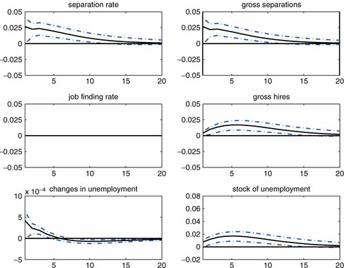
Contribution of the separation rate: fixed job finding rate and variable separation rate. Note: The shock is identified by imposing Restrictions 1 and 2. The black solid line represents the median of the posterior distribution. The error band represents the 16th and 84th percentiles of the posterior distribution. The response of changes in unemployment is expressed as a level deviation from the steady-state level (zero). Responses of the stock of unemployment and vacancies are expressed as log deviations from the steady-state levels. This figure is available in colour online at wileyonlinelibrary.com/journal/jae
Figure 6 considers what happens if the separation rate is fixed at the steady-state level while letting the job finding rate take the estimated actual paths. Note again that it is entirely possible that separations actually move due to the feedback effect from changes in the pool size ( = 1 − ut) driven by changes in the job finding rate. The top right panel shows that this is actually not the case; while gross separations do move due to the feedback effect, the effect is quantitatively minuscule. Moreover, when the separation rate is constant, declines in the job finding rate induce gross hires to decrease, which is highly counterfactual.
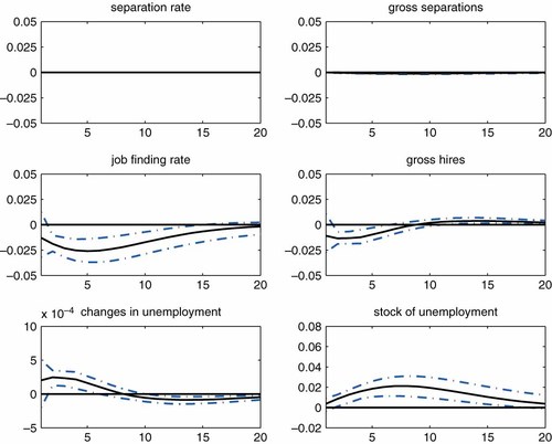
Contribution of the job finding rate: fixed job joss rate and variable job finding rate. Note: The shock is identified by imposing Restrictions 1 and 2. The black solid line represents the median of the posterior distribution. The error band represents the 16th and 84th percentiles of the posterior distribution. The response of changes in unemployment is expressed as a level deviation from the steady-state level (zero). Responses of the stock of unemployment and vacancies are expressed as log deviations from the steady-state levels. This figure is available in colour online at wileyonlinelibrary.com/journal/jae
The bottom right panels of Figures 5 and 6 present the unemployment response in the two hypothetical scenarios. Comparing the actual response shown in the bottom panel of Figure 3, one can observe that overall, both margins contribute equally to the unemployment responses. However, there are some differences in terms of the timing of the effects. The effects of the separation rate appear larger during the first year after the shock, while the effects of the job finding rate become more prevalent in the midst of the downturn.27
Although the exercise here is purely illustrative, it nonetheless sheds some light on the quantitative and qualitative importance of fluctuations in the two transition rates. In particular, it clearly suggests that both margins are quantitatively important and that ignoring movements of the separation rate produces highly counterfactual implications on the remaining variables.
3.4. Robustness
I examine the robustness of the results so far with respect to the following dimensions: (i) treatment of the deterministic trends; (ii) lag length; and (iii) horizon (K) for which changes in unemployment are restricted to being non-negative.
For (i), I consider three cases. The first two cases correspond to the linear detrending and no detrending (i.e., constants are the only deterministic variables of the VAR). The third case estimates the same model by restricting the sample up to the end of 1996. Recall that the reason for the use of quadratic trends in the benchmark specification is that the vacancy series and the separation rate series exhibit secular declines, which has been particularly pronounced since the mid 1990s. This subsample estimation is carried out with no detrending of the data. Figure 7 compares the median responses of two transition rates, unemployment and vacancies across these three cases together with those from the benchmark case. These impulse responses clearly indicate that specifications of the deterministic components have only little impact on the results.
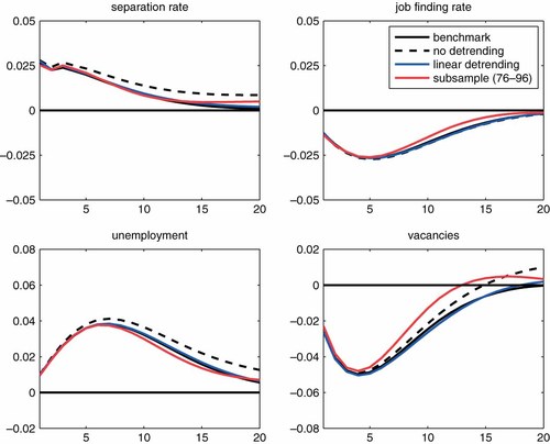
Robustness: alternative detrending methods and sample period. Note: The shock is identified by imposing Restrictions 1 and 2. Each line represents the median response for each specification. Responses are expressed as log deviations from the steady-state levels. This figure is available in colour online at wileyonlinelibrary.com/journal/jae
Figure 8 presents the results based on a lag length of four quarters (instead of two) and K = 4 (instead of 2). This figure also demonstrates that the benchmark results discussed above are not sensitive to these alternative specifications.
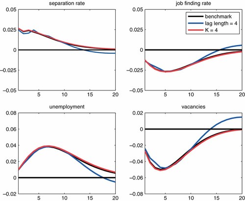
Robustness: alternative lag length and K. Note: The shock is identified by imposing Restrictions 1 and 2. Each line represents the median response for each specification. Responses are expressed as log deviations from the steady-state levels. This figure is available in colour online at wileyonlinelibrary.com/journal/jae
3.5. Expanded Model
So far I have been agnostic about the nature of the shocks that underly the Beveridge curve relationship. This subsection expands the VAR system and attempts to distinguish the underlying shocks. In the above analysis, I have established the usefulness of the benchmark model by showing that even with such a parsimonious system, dynamics of the labor market can be characterized with no sign ambiguity. Nevertheless, it is of economic interest to examine whether the different underlying shocks influence the labor market variables differently, and if so, how different the effects are. On the other hand, attesting to the similarity of the responses of the labor market variables adds to the confidence about the previous results. I expand the system by including the inflation rate and labor productivity growth.28 With this five-variable VAR, I identify the demand shock and productivity shock by imposing the following sign restrictions.
3.5.1. Demand Shock
Identification
To identify the demand shock, I impose a restriction on the price level behavior as well as the same Beveridge curve restrictions used above. Specifically, it is assumed that the expansionary demand shock raises the price level at least for four quarters and that it causes vacancies to rise in the first quarter and the unemployment change to be negative for the first two quarters.29 These restrictions are in line with the price–output restrictions used by Peersman (2005) and Braun et al. (2007). While I do not use an output variable directly, the unemployment rate, which is implicitly captured by the two transition rates, plays that role. I can also justify these restrictions on the basis of the properties of fully specified monetary DSGE models with search/matching frictions such as Cooley and Quadrini (1999), Walsh (unpublished, 2005) and Trigari (2009). The number of periods for which the price-level behavior is restricted is set to four quarters, following Braun et al. (2007). The results are, however, insensitive to the choice.
Results
The impulse response functions to the demand shock are shown in Figure 9. The qualitative pattern of the labor market responses is remarkably similar to the results from the benchmark case; both separation and job finding rates contribute roughly equally to the unemployment fluctuations. Relative to the benchmark case, the size of the responses is reduced roughly by half. The variance decomposition indicates that the demand shock explains roughly 20% of the variations in the labor market variables for all horizons.
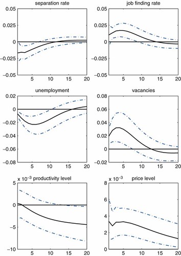
Impulse responses to the positive demand shock. Note: The shock is identified by imposing the price-level restriction and the Beveridge curve restrictions. See text for details. The black solid line represents the median of the posterior distribution. The error band represents the 16th and 84th percentiles of the posterior distribution. Responses are expressed as log deviations from the steady-state levels. This figure is available in colour online at wileyonlinelibrary.com/journal/jae
Turning to the non-labor-market variables, the responses of the price level exhibit strong persistence as is expected from the sign restriction.30 The short-run effects on labor productivity are ambiguous, but in the long run the shock tends to push down labor productivity. The latter result needs more thorough investigation, but it is consistent with standard production technology that exhibits decreasing returns to labor.
3.5.2. Technology Shock
Identification
A practice widely used in the literature to identify the technology shock is to apply the long-run restriction on labor productivity pioneered by Galí (1999). He shows that the technology shock lowers aggregate hours as opposed to the prediction of the standard RBC model. A recent paper by Dedola and Neri (2007) examines the robustness of Galí's finding by applying the sign restriction approach to identify the technology shock. Specifically, they assume that the technology shock raises the level of labor productivity over a long horizon (i.e., 20 quarters). I adopt this assumption together with the price-level restriction that the shock lowers the price level for four quarters.
Given the diverse findings in the literature on this issue, determining the direction of the response of unemployment with respect to the technology shock requires somewhat careful judgment. In all of the papers cited in Section 3.2, the technology shock takes the form of a disturbance to TFP of constant returns to scale technology of the representative matches (or jobs). In this case, as was discussed in that subsection, it is conceivable that the (positive) technology shock is associated with higher vacancies and lower unemployment (see Merz, 1995, and Andolfatto, 1996, as representative examples). However, a recent paper by Canova et al. (2007) develops a vintage model backed by the Schumpeterian view in which the relationship between the technology shock and unemployment is reversed (i.e., the technology shock causes unemployment to increase).31 This is because when new technology is introduced into the economy it prompts the cleansing of technologically obsolete jobs, raising the separation rate and thereby unemployment. Canova et al. (2007) argue that the vintage structure of their model is consistent with Galí's long-run identification and that the identified technology shock indeed raises unemployment.
Although theoretical consideration does not provide me with clear guidance regarding the unemployment response to the technology shock, I assume that the positive technology shock raises unemployment, following Canova et al. (2007).32 Alternatively, I could proceed with no assumption on the behavior of unemployment, and let the productivity and price restrictions alone tell whether unemployment is likely to rise or decline. However, this exercise did not yield unambiguous results; i.e., resulting unemployment responses include a wide range of possibilities, with the median response being close to zero. Thus, imposing a priori the positive relationship between the technology shock and unemployment is necessary.
Finally, I chose to impose no restrictions on the vacancy behavior, as opposed to the exercises so far. It appears that the vintage model in its simple form predicts that the technology shock leads to increases in vacancies. However, this implies that unemployment and vacancies are correlated positively. Thus, I simply let the data decide the vacancy response.33
Results
The results are presented in Figure 10. First, note that the responses of productivity and price levels are consistent with the results in the literature. Relative to the benchmark results shown in Figures 2 and 3, the responses of the labor market variables are somewhat less clear-cut. Also as in the case of the demand shock, the size of the responses is reduced roughly by half relative to the benchmark case. However, the overall pattern of the labor market responses again remains the same as before.
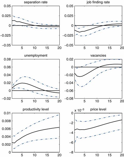
Impulse responses to the technology shock. Note: The shock is identified by imposing the restrictions on the price level, productivity level and unemployment. See text for details. The black solid line represents the median of the posterior distribution. The error band represents the 16th and 84th percentiles of the posterior distribution. Responses are expressed as log deviations from the steady-state levels. This figure is available in colour online at wileyonlinelibrary.com/journal/jae
Observe also that vacancies tend to drop in the face of the positive technology shock, suggesting that the negative relationship between unemployment and vacancies is quite strong in the data. Examining whether or not the empirical behavior of vacancies is consistent with the Schumpeterian vintage model seems to be an interesting issue to explore, but it requires a fully specified DSGE model, which is beyond the scope of this paper. Last, the variance decomposition reveals that the median contributions of the identified technology shock to variations in the three labor market variables amount to 10–15% over all horizons.
4. HETEROGENEITY IN THE DYNAMICS OF WORKER FLOWS
This section extends the benchmark model to address an important heterogeneity in the cyclicality of worker flows across different demographic groups. The heterogeneity arises when transitions into and out of the labor force are explicitly taken into consideration. While the previous analysis based on the aggregate transition rates between employment and unemployment seems to be of first-order importance given the current state of quantitative macro/labor literature, the results in this section point to an important direction for future research.
4.1. Motivation and the Method
This section is motivated by the results reported in Fujita and Ramey (2006), who find that the aggregate separation rate becomes far less countercyclical when NILF flows are incorporated into the analysis. We show that behind this is the composition effect that the separation rate of young workers becomes essentially acyclical when we treat the E-to-NILF flow as part of separations, whereas that of prime-age (25–54) workers, especially prime-age male workers, is strongly countercyclical regardless of the inclusion of the E-to-NILF flow. Motivated by these results, I estimate a VAR using disaggregated data across age and gender with inclusion of NILF flows.34 Having established that my previous results are robust with respect to alternative specifications and identification of different types of shocks, I maintain the identification scheme based on the Beveridge curve relationship only. I consider three age groups: young (16–24), prime-age (25–54), and old (55 or above), and therefore a total of six demographic groups are included in the analysis.
Incorporating the NILF flows


Aggregation and sign restrictions
I estimate the VAR model with those transition rates for six demographic groups and vacancies. There are therefore a total of 13 variables (i.e., two transition rates for each of the six demographic groups plus the aggregate vacancy series). All series are pre-detrended in the same way as in the aggregate model. I do not impose any restrictions on the cross-effects among those demographic groups. Lag length is set to two quarters.37

4.2. Results
Figure 11 presents the aggregate-level behavior of changes in unemployment, the stock of unemployment and vacancies. Although the magnitude of deviations from the steady-state levels is somewhat smaller in this disaggregate model (compared to corresponding results from the aggregate model), overall patterns of the responses are quite similar: both unemployment and vacancies exhibit hump-shaped responses.40
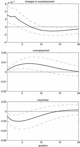
Aggregate-level responses of unemployment and vacancies from the disaggregate model. Note: The shock is identified by imposing Restrictions 1 and 2. The black solid line represents the median of the posterior distribution. The error band represents the 16th and 84th percentiles of the posterior distribution. Responses of unemployment and vacancies are expressed as log deviations from the steady-state levels. This figure is available in colour online at wileyonlinelibrary.com/journal/jae
Figure 12 plots unemployment responses for four (out of six) demographic groups.41 The four panels in the figure clearly indicate that the negative aggregate shock induces gradual positive responses in unemployment. Further, observe that the response of prime-age males is most pronounced among them.
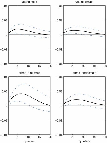
Unemployment responses for demographic groups. Note: The shock is identified by imposing Restrictions 1 and 2. The black solid line represents the median of the posterior distribution. The error band represents the 16th and 84th percentiles of the posterior distribution. Responses are expressed as log deviations from the steady-state levels. This figure is available in colour online at wileyonlinelibrary.com/journal/jae
Each of Figures 13 through 16 displays responses of the four variables—separation rate, gross separation, job finding rate and gross hires—for each of the four demographic groups. First, consider the responses of prime-age male workers, presented in Figure 15. The pattern conforms to the findings of the aggregate model that focuses on E/U transitions; the separation rate and gross separations are higher in the face of the adverse shock, while the job finding adjusts more slowly, and the number of gross hires increases because the pool of job seekers expands as more workers leave employment.
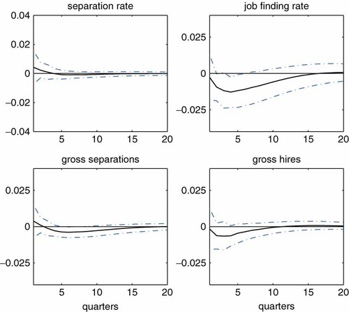
Responses of young male workers to the aggregate shock. Note: The shock is identified by imposing Restrictions 1 and 2. The black solid line represents the median of the posterior distribution. The error band represents the 16th and 84th percentiles of the posterior distribution. Responses are expressed as percentage deviations from the steady-state levels. Responses are expressed as log deviations from the steady-state levels. This figure is available in colour online at wileyonlinelibrary.com/journal/jae
Consider the other three groups of workers (Figures 13, 14 and 16). First, responses of the separation rates for these three groups of workers are not distinguishable from zero. Responses of the job finding rates show procyclicality across the board. Reflecting declines in the job finding rates, gross hires tend to become lower within a year after the shock occurs. Similarly, gross separations are more likely to be lower than higher.
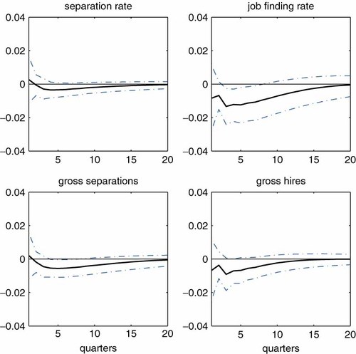
Responses of young female workers to the aggregate shock. Note: The shock is identified by imposing Restrictions 1 and 2. The black solid line represents the median of the posterior distribution. The error band represents the 16th and 84th percentiles of the posterior distribution. Responses are expressed as log percentage deviations from the steady-state levels. Responses are expressed as log deviations from the steady-state levels. This figure is available in colour online at wileyonlinelibrary.com/journal/jae

Responses of prime-age male workers to the aggregate shock. Note: The shock is identified by imposing Restrictions 1 and 2. The black solid line represents the median of the posterior distribution. The error band represents the 16th and 84th percentiles of the posterior distribution. Responses are expressed as log deviations from the steady-state levels. This figure is available in colour online at wileyonlinelibrary.com/journal/jae
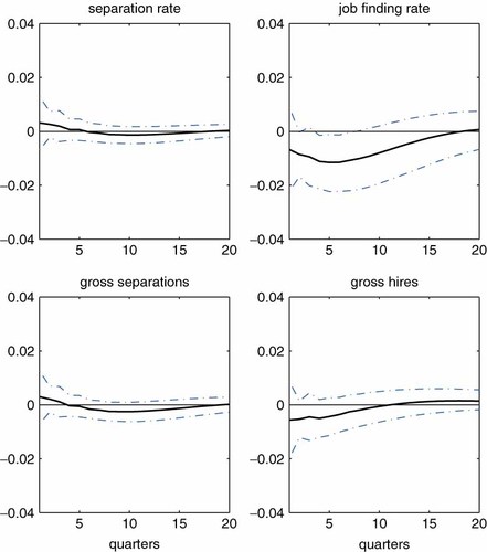
Responses of prime-age female workers to the aggregate shock. Note: The shock is identified by imposing Restrictions 1 and 2. The black solid line represents the median of the posterior distribution. The error band represents the 16th and 84th percentiles of the posterior distribution. Responses are expressed as log deviations from the steady-state levels. This figure is available in colour online at wileyonlinelibrary.com/journal/jae
The results for these groups of workers indicate that slower job finding during recessionary periods drives the worker reallocation process. Consider a hypothetical case similar to one of the two scenarios considered before, where the job finding rate is lower, while the separation rate is simply constant. In this case, as studied in Figure 6, gross hires decline as a direct consequence of slower job finding, eventually causing declines in employment. The constant separation rate then implies lower gross separations.
When I estimate the disaggregate model with E/U transitions only, I find that all demographic groups show the same pattern as in the aggregate model. The results in this section therefore suggest that the participation decision plays an important role in understanding the cyclical adjustments among the groups other than the prime-age male workers. On the other hand, robustness of the results among prime-age male workers with respect to inclusion of NILF flows carries a large weight in thinking about the stylized facts of US labor market dynamics from macroeconomic perspectives, since those workers tend to be in long-term, high-wage jobs. Further discussions on this issue can be found in Fujita and Ramey (2006, Section 9), who find similar results.
5. CONCLUSION
This paper has applied structural VARs with sign restrictions to uncover robust dynamic features of the US labor market. In line with the results by Elsby et al. (2009), Fujita and Ramey (2006, 2009), Fujita et al. (2007) and Yashiv (2007), I have shown that countercyclicality of separation is a quite robust feature of the data and is important in accounting for unemployment dynamics, as opposed to the views put forth by Shimer (2007) and Hall (2005a,b). In particular, I have argued that the observed countercyclical feature of gross hires could not have arisen unless the effects of the separation rate on unemployment dynamics are strong enough. I have also shown that the same results hold with respect to different kinds of shocks.
Given the robustness, these results should be taken seriously in the quantitative macro/labor literature. The first obvious message from the results is that the models with exogenous separation miss an important part of the story behind unemployment dynamics, and thus future research should consider the models with the endogenous separation decision. Second, the responses of vacancies and the job finding rate always exhibit a hump-shaped pattern. This robust feature of the data cannot be replicated in the standard search/matching model, whether the separation decision is exogenous or endogenous, owing to the rapid responses of vacancies in the model.42 In Fujita and Ramey (2007), we extend the standard search/matching model (with a fixed separation rate) by introducing sunk job creation costs that are incurred when new jobs are created. This extension makes vacancies a predetermined variable (instead of a jump variable as in a standard model), generating more realistic dynamics in vacancies and unemployment. Extending it to the environment with endogenous separation is an important step going forward.
The last section estimated the disaggregate model using the data disaggregated by six demographic groups and incorporating transitions into and out of the labor force. The separation rate continues to play a dominant role among prime-age male workers, while for other groups changes in the job finding rate are more important. While the main results based on the aggregate transition rates between employment and unemployment seem to be of first-order importance, explicitly considering worker heterogeneity and the participation decision in the labor matching framework certainly contributes to a deeper understanding of US labor market dynamics.
ACKNOWLEDGMENTS
I am grateful for useful comments from or discussions with Craig Burnside, Hal Cole, Wouter den Haan, Chris Foote, Jim Hamilton, Giorgio Primiceri, Garey Ramey, Juan Rubio-Ramirez, Frank Schorfheide, Keith Sill, Harald Uhlig, anonymous referees and seminar participants at various places. All remaining errors are the author's. The views expressed here do not necessarily reflect those of the Federal Reserve Bank of Philadelphia or the Federal Reserve System.
REFERENCES
 .
.
 without considering gross flows. The right-hand side is often called the conditional steady-state value because it gives the unemployment rate that would prevail when the transition rates stay at st and λt. Shimer (2007) shows that the behavior of the actual unemployment rate is well approximated by the conditional steady-state values. See Pissarides (1986) for the same exercise in Britain. This, however, does not necessarily imply that behavior of gross flows is irrelevant for understanding labor market dynamics, as argued elsewhere in this paper.


