How much between-group wage gaps can be explained by talent allocation frictions in China?
Abstract
What explains huge wage gaps between different hukou and gender groups in China? This paper uses an overlapping generation model with human capital investment and occupational choices to quantify how much wage gaps between these groups can be imputed to two types of talent allocation frictions, labor market discrimination, and human capital accumulation barriers. The calibrated model indicates that the two types of talent allocation frictions can explain a significant proportion (four-fifths, one-third, and three-fifths) of the wage gap between each non-urban-men group (urban women, rural men, and rural women) and urban men in 2013. Our counterfactual exercise also shows that eliminating these two frictions since 1995 would result in about half a percentage point increase in China's economic growth rate between 1995 and 2013.
1 INTRODUCTION
Recent studies documented huge urban–rural and gender income gaps in China (Ge & Zeng, 2011; Huang, 2019; Li et al., 2014; Wang, 2005b). To explore the gender wage gap and the wage gap between urban and rural workers simultaneously, we divide workers into four groups, urban men, urban women, rural men, and rural women.1 Using data from the China Household Income Panel (CHIP), we find that the average wages of urban men are significantly higher than those of the other three groups in China. In 2013, the average wages of urban women, rural men, and rural women were only about 80%, 70%, and 40% of that of urban men respectively. What contributes to such huge wage gaps between different hukou and gender groups is an important issue.2
Exploring the causes of the between-group wage gaps is not only of theoretical interests, but also has practical significance: the wage gaps not only directly affect the welfare of the disadvantaged groups, but also affect economic growth through resource allocation channels. Targeting at the frictions that are responsible for the wage gaps, government policies can improve the efficiency of workers' allocation and narrow the between-group wage gaps simultaneously.
In this paper we examine two main causes of the wage gap between groups: berries to human capital accumulation and discrimination in the labor market, which two are collectively referred to as talent allocation frictions. These frictions can affect the average wages of disadvantaged groups through direct and indirect channels. In both the direct and indirect channels, workers' decisions on human capital investment and occupational choices are the key to transmit the frictions.
To implement the scheme above, we use the model of Hsieh et al. (2019) to make both the human capital investment and occupational choices endogenous and provide a model-based quantification of the contribution of the two talent allocation frictions to between-group wage gaps in China. As in Hsieh et al. (2019), the model in this paper uses an occupation-specific wedge between wages and marginal products to capture the labor market discrimination. This wedge is a proxy for gender (hukou) inequalities in employment (hiring discrimination) and different pay for equal work (wage discrimination). Also as in Hsieh et al. (2019), the model in this paper lets accumulating occupation-specific human capital be associated with increased monetary costs to capture barriers to human capital accumulation. These costs are a proxy for differences in school quality between rural and urban areas, parental and teacher discrimination in girls in the development of certain skills, and any other factors that may hinder equal opportunity in primary and secondary education. The agent's decisions on human capital investment and occupational choice are affected by five factors: talents of her/his own, occupational preferences and human capital endowments of her/his group, barriers to human capital accumulation, and labor market discrimination suffered by her/his group. Given the above setup, a disadvantaged group will expect to face the corresponding discrimination if they choose a kind of occupation and that the return of human capital investment varies with occupations. Therefore, the model used in this paper permits us to take into account the impact of talent allocation frictions on human capital accumulation and occupational distribution. To quantitatively evaluate the fraction of the between-group wage gaps caused by talent allocation frictions, the disparity between the true between-group wage gaps in data and the counterfactual between-group wage gaps without talent allocation frictions are calculated.
Using micro-data from CHIP, under a series of standardizations and identification assumptions, we can use our model to back out the human capital accumulation barriers and labor market discrimination that urban women, rural men, and rural women suffer in each occupation. Through a series of counterfactual exercises, we can answer the questions of interest: the two types of talent allocation frictions can explain how much wage gaps between different hukou and gender groups in China, and which type of frictions seriously affects a certain disadvantaged group.
We find that the two types of talent allocation frictions faced by urban women (rural women) can explain four-fifths (three-fifths) of the wage gap between them and urban men in 2013 and that labor market discrimination and barriers to human capital accumulation both played important roles in explaining the wage gap. The two talent allocation frictions faced by rural men can explain about one-third of the wage gap between them and urban men in 2013, the obstacle to human capital accumulation suffered by them played a leading role in explaining the wage gap, but (negative) labor market discrimination faced by them narrowed the wage gap.
To show how severe the output cost resulting from talent allocation frictions is, we also calculate the counterfactual economic growth if these frictions were eliminated. We find that if there were no talent allocation frictions since 1995, the economic growth rate between 1995 and 2013 would have been about half a percentage point higher.
Our paper is closely related to Hsieh et al. (2019). We use their framework to study the contribution of talent allocation frictions in the Chinese labor market to wage gaps between groups of different hukou and gender, while Hsieh et al. (2019) examined the effect on the U.S. aggregate productivity of the improved allocation of talent over different occupations (caused by changes in talent allocation frictions) between 1960 and 2010. In the model of Hsieh et al. (2019) talent allocation frictions present themselves as aggregate measures, which vary with groups but do not vary with individuals within a group. This setup makes the framework in Hsieh et al. (2019) applicable to any economy with different groups that face different talent allocation frictions, despite the fact that the causes for talent allocation friction can vary from economy to economy. Although we take the framework of Hsieh et al. (2019), there is a key difference between our model and theirs. For Hsieh et al. (2019), the relative human capital endowment between groups does not affect their research results since they focus on the aggregate productivity. But in our model, the difference in human capital endowments is one of the causes of the between-group wage gap. Therefore, we cannot assume that human capital endowment is the same for different groups as Hsieh et al. (2019) do, and we must calibrate the relative human capital endowment (see Section 4.3).
Our research is also related to the following three branches of literature. The first branch of literature focus on measuring the impact of labor market discrimination (both wage and hiring discrimination) on between-group wage gaps (Guo & Zhang, 2012; Li, 2008; Li & Ma, 2006; Meng & Zhang, 2001; Wang, 2005a; Wu & Wu, 2009; Yu & Chen, 2012). According to this literature, the between-group wage gap can be decomposed into four exogenous and independent components: the within-occupation earnings differential due to the difference in endowment, the within-occupation earnings differential due to wage discrimination, the portion of the wage gap that can be explained by the difference in occupational distributions, and the portion of the wage gap due to recruitment discrimination. Our paper complements this literature by endogenizing human capital investment and providing micro-foundation for the occupational distribution of a group. It is reasonable to predict that labor market discrimination may affect the human capital investment of the discriminated group3, which will affect their accumulation of human capital and average wage. This channel through which discrimination affects the average wage is ignored by the econometric decomposition method, which will underestimate the contribution of discrimination to the wage gap.
The second branch of literature is about exploring the impact of human capital accumulation barriers on between-group wage gaps (Chen et al., 2010; Han & Fu, 2014; Jin & Gao, 2007; Lv et al., 2015; Wen, 2007; Yang et al., 2008).4 This group of literature focuses on some specific forms of human capital accumulation barriers faced by rural areas, such as the difference in government educational investment between urban and rural areas which leads to lower quality of rural education. They have ignored other forms of human capital accumulation obstacles faced by rural workers. The barriers to human capital accumulation in our paper are a comprehensive measure that can cover various specific forms of barriers to human capital accumulation. In addition, girls are more likely to suffer from barriers to human capital accumulation than boys in China, which is also completely ignored by the studies on the causes of the gender wage gap.
Compared with the above two branches of literature, our paper also has the advantage to incorporate both the labor market discrimination and human capital accumulation obstacles into a unified analysis framework, which makes it easier for us to identify which kind of talent allocation friction is the main cause for the wage gap between a certain disadvantaged group and urban men. This is conducive to formulating more targeted policies and effectively narrowing the wage gap. Different from the literature, our paper also makes the following two adjustments. Using time series data from 1995 to 2013, our paper presents the trend of talent allocation frictions suffered by a certain disadvantaged group. Dividing workers into four groups based on both hukou and gender,5 we discover some new facts about between-group wage gaps in China. For example, we find that rural women suffer much higher talent allocation friction than urban women, while this is not the case for rural men.
The third branch of literature is related to evaluating the impact of talent allocation (Baumol, 1990; Celik, 2018; Hsieh et al., 2019; Hu & Shi, 2016; Ji, 2019; Li et al., 2017; Li & Yin, 2014; Murphy et al., 1991). The existing literature focuses on the impact of talent allocation across different economic activities on economic growth. Our paper emphasizes that talent allocation affects between-group wage gaps as well: when two groups face different talent allocation frictions over various occupations, their occupational distribution will be differentiated, and it in turn causes a disparity in their average wages.
This paper is divided into seven sections. The second section setups and solves the model. The third section describes the data used. The fourth section calibrates the model. The fifth section reports the results. The sixth section conducts a variety of robustness checks. The seventh section concludes.
2 MODEL
2.1 Model setup
The model used in this paper is an overlapping generation model nesting occupational choices, which follows Hsieh et al. (2019). Three factors influencing workers' occupational choices and human capital accumulations are added to the traditional occupational choice model: labor market discrimination, human capital accumulation barriers, and occupational preferences. The economy consists of  discrete occupations, one of which is a home sector. There are three types of agents in the economy: workers, final goods producers, and educational goods producers. They sell human capital, final goods, and educational goods, respectively, in competitive markets. Each worker works in one of the
  occupations. Workers have heterogeneous talents in these occupations. The fundamental allocation problem in this economy is how to match workers with occupations.
2.1.1 Workers
Workers are divided into four groups according to hukou status and gender. A worker chooses an occupation and invests in human capital on the chosen occupation in the pre-period (born to 25 years old, standardized to 1). She/he will work in the chosen occupation for the next four periods (determined by the characteristics of the data used), and during all these periods her/his engaged occupation and human capital investment are assumed to be fixed.
 6 and cohort c
  that chooses occupation i
  is
is
 ()
() is the worker's consumption in period t,
  is the time that the worker spends on human capital accumulation in the pre-period, and
  is the preference of the worker's group for occupation i. The trade-off between consumption and leisure is parameterized by
  ,
,  . For simplicity, there is no discount between periods. Here, the occupational preference of a group,
  , may not represent the true preference of the group to the occupation, but reflects what they perceive after the policymakers' intervention. For example, if policymakers think that rural men/women should stay in their hometown and engage in agricultural production, then rural men/women will have a high preference for the farmer (It is possibly due to some policy intervention like tax or subsidy).
 ()
()Here,  is the human capital endowment of group g in occupation i, which “reflects any differences in talent common to a group in a given occupation” (Hsieh et al., 2019);
  is only a function of age
  and reflects the impact of experience on human capital;
  is the occupation-specific return of time investment in human capital accumulation;
  is the goods that the worker invests in human capital accumulation in the pre-period, which requires the worker to repay throughout his or her working lifetime;
  is the elasticity of human capital with respect to the goods invested in human capital accumulation.
 ()
() captures the discrimination suffered by the worker's group in the labor market of occupation i in period t,
  is the talent of the worker in occupation i,
  is the skill level of the worker in period t,
  is the price of skill in the labor market of occupation i in period t. Hence,
  is the worker's net income in period t. In the second term in the right hand side of Equation (3),
  is the repayment of human capital goods investment by the worker in period t, and
  captures the obstacles faced by the worker in accumulating human capital. The worker borrows
  in the pre-period to purchase
  units of human capital goods investment. The loan is repaid throughout the worker's working life, so
 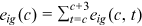 .
. occupations are subject to a multivariate Fr
 chet distribution:
 ()
() determines the dispersion of talents: the larger
  is, the smaller the dispersion is. The talent combination
  of a worker from group g can be seen as a realization of the multivariate Fr
 chet distribution.
For simplicity, we assume that individuals anticipate that the return to experience varies by age but that the labor market discrimination,  , returns to skill,
  , and returns to time investments in human capital,
  , will remain constant over time.
The timing of a worker's actions is as follows. Before entering the labor market, she/he knows her/his talents in all occupations and observes returns to skill, returns to time investments in human capital, obstacles to human capital accumulation and the labor market discrimination suffered by her/his group, which are expected to maintain at the level she/he observes at the beginning. Based on what she/he observes, the worker chooses the occupation that she/he will engage in and decides on the level of time and goods investment in human capital accumulation in the chosen occupation. The worker enters the labor market after reaching the working-age and will work for four periods in her/his chosen occupation. In this market, she/he will meet with, work for, and earn a wage from a final goods producer. The wage will be used for consumption after repaying the goods investment in human capital accumulation.
2.1.2 Final goods producers
 technology. Final goods are sold to workers for consumption and to educational goods producers to produce educational goods. The production function of a representative firm producing the final goods is
 ()
() is the exogenous productivity of occupation i,
  is the total efficiency units of labor in occupation i provided by group g (human capital), and
  is the elasticity of substitution across occupations in aggregate production.
 ()
() is the utility losses of the representative owner from hiring workers from group g in occupation i.
2.1.3 Educational goods producers (Schools)
 ()
() is the price of the educational goods
  ,7 and
  is the utility losses of the school owner due to providing educational goods of occupation i to workers from group g.
2.2 Model solution
2.2.1 Solving workers' problems
The worker's optimization problem can be solved in two steps, using backward induction method. The worker first calculates the maximized lifetime utility given any occupation by optimally choosing her/his choice variables: the level of time and goods investment in human capital, the consumption, and the loan repayments. The worker then goes back to see which occupation gives her/him the largest lifetime utility.
Optimal choices for a given occupation


 and
and 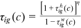 .
.Three assumptions are made to make the optimization problem analytical. First, we use a logarithmic utility function and assume that there is no discount between periods,8 which leads to that the optimal consumption of each period is equal. Next, we assume that the individual expectation for the future is as follows: except for experience accumulation, the variables that affect each period's income do not change over time. Such expectation, together with the logarithmic utility function, make the worker expected lifetime income a certain multiple of his/her income in the young stage. The solution for the workers' optimization problem is provided in Supporting Information: Appendix A.1.
Human capital time investment (schooling) is carried out before entering the labor market. The 25 years of worker time before entering the labor market are treated as one period and the workers make their schooling decision in this period. Schooling brings disutility to the worker by reducing leisure, but it increases lifetime income and each period's consumption by building up human capital. The worker optimal human capital time investment is given by  , where
  reflects the trade-off between consumption and leisure, and
  is the occupation-specific return of time investment in human capital accumulation.
Human capital goods investment is also carried out before entering the labor market, which is financed by borrowing.9 After entering the labor market, workers use some of their income to repay debts incurred by purchasing educational goods, while the rest is used for consumption. The cost of human capital goods investment increases debt that must be repaid in the future and it causes the consequent decrease in consumption. The benefit of human capital goods investment is the increase in human capital and the resulting increase in lifetime income and consumption. The greater the barrier to human capital accumulation, the smaller the increase in human capital level. The more discrimination is in the labor market, the smaller the increase in income brought about by the increase in human capital. Therefore, optimal human capital goods investment is declining in human capital accumulation obstacles and labor market discrimination. The optimal human capital goods investment is given by  .
.

 . The maximum utility of a worker in a given occupation is determined by the talent of the worker in that occupation,
  , and a comprehensive wage item,
  . Note that, the denominator of the comprehensive wage item is a composite item of two talent allocation frictions
  .
.Occupation choice

Given the optimal choices of workers provided in the above two steps, we can then analyze the distributional and aggregate variables in the labor market.
Occupational distribution
 ()
()Average skill
 ()
() .
.Average wage

 and
and  .
.Relative occupational propensity
 ()
()The solving processes of occupational distribution, average skill, average wage, and relative occupational propensity are shown in Supporting Information: Appendix A.2–A.5.
Wage gap

 is the average wage of group g in period t.
The wage gap between two groups is caused by the differences in two talent allocation frictions that they face, human capital endowments, and occupational preferences. The labor market discrimination suffered by a certain group affects the average wage of that group through three channels. First, the labor market discrimination will directly affect the wages received by individuals in this group, which is called the direct wage effect. Given the human capital accumulated in certain occupation,  , the more severe the labor market discrimination suffered by the group in the occupation, the lower the wages the individuals in this group will receive in this occupation. Second, the labor market discrimination will affect the wages received by individuals in this group indirectly by affecting the level of human capital accumulated, which is called the human capital accumulation effect. The more serious the labor market discrimination suffered by the group in the occupation, the lower the level of human capital the group will accumulate in this occupation. Third, the labor market discrimination will affect the average wage of the group by influencing the efficiency of the allocation of talent across occupations, which is called the talent allocation effect. The more dispersed in the
  occupations the labor market discrimination suffered by the group, the lower the efficiency of the allocation of talent and the lower the average wage of the group.
To understand the talent allocation effect, let's imagine that there is a group who does not face any human capital accumulation obstacles, but suffers from labor market discrimination, and has the same preference for all occupations. If the group suffers the same labor market discrimination in all occupations, the labor market discrimination is equivalent to a uniform wage tax. Regardless of the degree of labor market discrimination, all workers in the group will choose their occupations according to their own comparative advantages. The occupation distribution of the group is the same as that when the group does not suffer any labor market discrimination. Only when the group suffers different discriminations in different occupations, the occupational distribution of the group is different from that obtained when all occupations are not discriminated against. In other words, only when a group suffered different discrimination in different occupations would the group have talent misallocation. In summary, the obstacles to the accumulation of human capital affect the average wage of a group through the human capital accumulation effect and the talent allocation effect, while occupational preferences affect the average wage of a group only through the talent allocation effect.
2.2.2 Solving final goods producers' optimization problems
Because all employers are assumed to have the discriminative preferences over different groups of workers, perfect competition implies that  . When the owner of a final goods producing firm employs workers from a group that she/he discriminates against, she/he needs to be compensated for her/his utility loss via offering a lower wage to these workers. In equilibrium the lower wage exactly offsets the utility loss.


2.2.3 Solving schools' optimization problems
Perfect competition ensures that  and that
  . When the school owner provides educational goods
  to workers from a group that she/he dislikes, she/he needs to be compensated for her/his utility loss via asking these workers for a higher price. In equilibrium the higher price exactly offsets the utility loss. With prefect competition, the school owners earn zero profit, and
  .
.
2.3 Equilibrium
2.3.1 Definition of equilibrium
 , total efficiency units of labor in each occupation
  , final output
  , and prices, the efficiency wages
  , such that
- 1.
Given an occupation choice, idiosyncratic ability in that occupation
 , and the occupational wage
  , each individual chooses
  to maximize her/his expected lifetime utility given by (1) subject to the constraints given by (2), (3), and
  .
. - 2.
Each individual chooses the occupation that maximizes her/his expected lifetime utility, taking as given
 .
. - 3.
For a given group, given the talent distribution described by Equation (4), the occupation distribution is given by Equation (8), which sums to one over all occupations, and the average human capital in a given occupation is given by Equation (9), which sums to
 over all active cohorts.
 - 4.
Total output
 is given by the production function in Equation (5).
 - 5.
A representative firm in the final good sector hires
 in each occupation to maximize the utility given by Equation (6), taking efficiency wages as given.
 - 6.
School owners maximize the utility given by Equation (7).
- 7.
Perfect competition in the final goods and educational goods sectors ensures that
 and
and  .
. - 8.
The wage rate
 clears the labor market for each occupation.
The model in this paper is a “static” equivalent one in every period, but the equilibrium is not stationary. Two assumptions in our paper, as in Hsieh et al. (2019), transform the overlapping generation model into a “static” equivalent model. First, occupational choice and the goods and time investment in human capital are made before entering the labor market and remain unchanged upon entering the labor market. Second, when making the occupational choice and human capital investment decision, the individuals expect that the variables that affect each period's income remain at the level when young, except for experience accumulation. As a result, future variables are not included in the current period's equilibrium.
In each period, there are four active cohorts, one young cohort, and three older cohorts. The older cohorts' occupational distributions and human capital investments are unchanged after they enter the labor market, which also preset their current human capital supply in various occupations. The occupational distribution and human capital investment of the young cohort are endogenously determined by the current economic environment (labor market discrimination, human capital accumulation barriers, occupational preference, technology, and the human capital supply of the older cohorts), but not affected by the future economic environment. Consequently, the choices of the young cohort are “static” equivalent, and so does the occupational distribution of the young cohort. However, the economic environment differs from period to period, which makes the equilibrium nonstationary over time.
2.3.2 System of equilibrium equations
 ()
() ()
() ()
() ()
() ()
() ()
() ()
() represents the set of all active cohorts in period t and
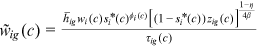
  is the number of workers from group g and cohort c. Equation (11) is the production function of final goods. Equation (12) is the demand function of human capital. Equation (13) is the supply function of human capital. Equation (14) describes the average quality of workers from group g and cohort c who chooses occupation i. Equation (15) describes the occupational distribution of workers from group g and cohort c. Equation (16) defines the comprehensive wage item in
  . Equation (17) defines the denominator of
  .
.3 DATA
The data used in this paper comes from the CHIP. Among all the available data, we use CHIP1995, CHIP2002, CHIP2007, and CHIP2013, but not CHIP1988, since the later does not contain the information on the changes in hukou status.
There are 12 kinds of occupations in this paper: the home sector, engineering technical personnel, teachers and tutors, health technical personnel, other professional and technical personnel, clerk and related personnel, commercial and service workers, farmers, manufacturing workers, transport equipment operation and related workers, construction workers, and other production and transport equipment operation and related workers.10
Workers are divided into four groups based on hukou status and gender: urban men, urban women, rural men, and rural women. The group of rural workers include both workers who have been holding agricultural hukou since birth and workers who held an agricultural hukou from birth to at least 16 years old and had changed to urban hukou for various reasons such as being admitted to a college, or joining the army and becoming an officer, or being recruited as a worker in urban areas. These rural workers who have changed their hukou held agricultural hukou for most of the time before entering the labor market and were mainly educated in rural primary and secondary schools in childhood. Relative to workers who have been holding urban hukou since birth or converted to urban hukou at younger ages, these rural workers may suffer more human capital accumulation barriers and been discriminated against in the labor market. Accordingly, we have the following definition of urban/rural workers. The hukou registration history of workers can be roughly divided into the following three types: having been holding agricultural hukou since birth, changing from agricultural hukou to urban hukou, and having been holding urban hukou since birth. Workers who have been holding agricultural hukou since birth are rural workers. Workers who have been holding urban hukou since birth are urban workers. Workers who switched their hukou status from agricultural hukou to urban hukou after 16 years old are rural workers. In each year's urban questionnaire, these switched rural workers accounted for about one-fifth of all workers. If these switched rural workers were classified as urban workers, we will underestimate the fraction of rural workers in non-farmers occupations, especially in professional and technical occupations, and overestimate the frictions they face in those occupations. Workers who switched their hukou status from agricultural hukou to urban hukou before 16 years old are urban workers.
We focus on workers in the 26–49 age group. We assume that workers receive education before 26 years old and cannot return to school after entering the labor market. The legal retirement age for female workers in the public sector in China is 50 years old. To avoid retired workers, only workers under 50 years old are analyzed. Corresponding to the interval of years of the data used in this article, each cohort spans 6 years. The working life of a worker will go through four stages: 26–31 (Young), 32–37 (Middle Young), 38–43 (Middle Old), 44–49 (Old).
Individuals in the model survive for four periods. Each period lasts 6 years. The notation  indicates the cohort considered, the notation
  indicates the year (data) that the cohort is now living, and
  gives the cohort's life stage. This is consistent with the CHIP data that we use. The data structure used in our paper is similar to that of Hsieh et al. (2019). CHIP data from 1995, 2002, 2007, and 2013 are used, and the time interval between adjacent CHIP data ranges from 5 to 7 years. The cohort born between 1964 and 1969 is young in CHIP1995, becomes middle-young in CHIP2002, middle-old in CHIP2007, and old in CHIP2013. Therefore, this cohort happens to live a complete life cycle in the data that we use. In each CHIP data, there are four active cohorts. For example, in CHIP2013, the cohort born between 1964 and 1969 is old, the cohort born between 1970 and 1975 is middle-old, the cohort born between 1976 and 1981 is middle-young, and the cohort born between 1982 and 1987 is young.
In the data processing, three adjustments are made: first, the number of urban workers is adjusted according to the urbanization rate of the hukou registration population; second, the contribution of land is deducted from farmers' income; third, the change in price levels is deflated using CPI. The reasons are as follows. There are generally three questionnaires in each wave of survey: urban questionnaire, rural questionnaire, and immigration questionnaire. The sample size of the urban questionnaire does not reflect the urbanization level of the hukou registration population. There were too many urban workers in the early years of the survey, and there were too few urban workers in the later years of the survey. To correct this inconsistency, we adjust the number of urban workers based on the urbanization rate of the hukou registration population. Some of the farmers' income comes from land. We only consider labor income here, so the contribution of land is deducted from farmers' income.
We aim to get three moments from the data: average wage  , occupation distribution
  , and average years of education
  , for all
  . These moments are used to calibrate the model.
4 CALIBRATION
The value of the following parameters need to be calibrated:  , for all
  .
.
4.1 Identification assumptions and normalization
Our first task is to use the panel data on occupational distribution,  , and wages,
  , from 1995 to 2013 to uncover the change in two talent allocation frictions,
  and
and  , and preferences,
  . To do so, the following assumptions are made. Some of these assumptions are already embedded in our model setup: occupational talents are distributed i.i.d. Fr
 chet; the human capital time and goods investments of workers are only made before entering the labor market; labor market discrimination affects all cohorts of a group in the labor market equally at the same point of time. One additional identification assumption is that the relative human capital endowment of women and rural workers to urban men is constant over time.
To identify the relative human capital endowment  , we need some further assumptions and standardization on the human capital endowment. The human capital endowment of urban men in each occupation is normalized to one, that is,
  , for all
  . We assume that other groups have the same human capital endowment as urban men in the home sector and commercial and service sectors, that is,
  , for
, for  home or commercial and service workers and all
  , although
  for other 10 occupations are allowed to be different from
  . The other 10 occupations are divided into two sets. One set is called Brain occupations (denoted as Brain), which include engineering technical personnel, teachers and tutors, health technical personnel, other professional and technical personnel, and clerk and related personnel. The other set is called Brawn occupations (denoted as Brawn), which include farmers, manufacturing workers, transport equipment operation and related workers, construction workers, and other workers. In the benchmark model, we assume that urban (rural) workers have the same human capital endowment in Brain occupations, that is,
  , and
, and  , for all
  . We assume that women (men) have the same human capital endowment in Brawn occupations, that is,
  , and
, and  , for all
  . These assumptions are made with a general sense that (1) people are born with an Intelligent Quality that is drawn from a common distribution if they are all born in a city (in a rural area) and that (2) women and men are born differently in terms of physical strength.11
Next, we need to pick one sector and one group as being undistorted. The home sector and urban men are selected as the undistorted sector and the undistorted group respectively. In the calibration process, we should consider the fact that no urban worker takes the farmer as her/his occupation. Based on these considerations, we make the following identification assumptions and standardization: all groups are undistorted in the home sector and all groups' preferences for the home sector are standardized to 1, that is,  ,
,  and
and  ,
,  ; urban men are undistorted in all occupations except farmers and their preferences for these occupations are all normalized to 1, that is,
  ,
,  and
and  ,
,  ; to calibrate farmer related parameters, it is assumed that rural men do not face any distortions as farmers, that is,
  and
and  ,
,  ; to fit the fact that no urban worker takes the farmer as her/his occupation, it is assumed that urban workers do not face any distortions as farmers and their preference for farmers is 0, that is,
  ,
,  ,
,  ,
,  ,
,  and
and  ,
,  ,
,  .
.
The identifying assumptions and normalization for our parameterization of the model are summarized in Table 1.
| Parameter | Definition | Value |
|---|---|---|
 |
Human capital accumulation barriers | 0 |
 |
Labor market discrimination | 0 |
 |
Innate talent | 1 |
 |
Innate talent in home sector | 1 |
 |
Innate talent as commercial and service workers | 1 |
 |
Home human capital accumulation barriers | 0 |
 |
Home labor market discrimination | 0 |
 |
Occupational preferences for farmers | 0 |
 |
Occupational preferences for farmers | 0 |
 , ,  |
Occupational preferences | 1 |
 |
Home occupational preference | 1 |
4.2 Estimation of  ,
,  ,
,  , and
, and 
To identify beta, we use  , which follows the argument in Hsieh et al. (2019) that the Mincerian return
  of more or less 1 year around mean schooling
  should satisfy
 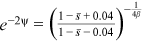 . We obtain the Mincerian return across occupations from a regression of log average wages on average schooling across occupation-groups, with group dummies as controls. We choose
  , the average of the estimated
  values across years.
Since  is the share of education expenditure in labor income, we can identify its value by finding its counterpart in the data. According to the education expenditure data provided by the China Education Statistical Yearbook and the GDP data provided by the China Statistical Yearbook, the average share of education expenditure in GDP in the 4 years we focus on is
  . According to Wang and Yuan (2018), the average share of labor income in GDP in the same 4 years is
  . Therefore, we set
  as our baseline value.
Given our assumptions, the distribution of wages within an occupation for a given group is Fr chet, whose shape parameter is
  . The shape parameter estimated by Ji (2019) is 4.32. Accordingly,
  . In our benchmark case,
  . Following the literature, we set the elasticity of substitution between different occupations at
  in our baseline model. In Section 6, we will explore the robustness of our results to other values of
  .
.
The values of these key parameters are summarized in Table 2.
| Parameter | Definition | Determination | Value |
|---|---|---|---|
 |
Fr chet shape chet shape |
Wage dispersion, Frisch elasticity | 5 |
 |
Goods elasticity of human capital | Education spending share in labor income | 0.074 |
 |
Elasticity of substitution across occupations | Literature | 3 |
 |
Consumption weight in utility | Mincerian return to education | 0.1724 |
4.3 Calibration of frictions and human capital endowment
 , we get the following equation:
 ()
() and
and  , from Equation (10), using the following identification assumptions:
  ,
,  , and
, and  . The left side of Equation (18) is the ratio of composite friction term to human capital endowment. The right side of Equation (18) contains relative employment propensity and relative wage of young. Average wage
  and occupation distribution
  can be obtained from the data used in this paper.
To identify the composite friction term  , we also need to know human capital endowment
  . The right side of Equation (18) is denoted as
  . We denote the minimum of
  that (young) rural workers have in Brain occupations in 2013 as
  . Denote the group (occupation) having
  as
as  (
( ). We assume that the young worker in group
  does not face any talent allocation friction in occupation
  in 2013, or equivalently assume that the differences in employment share and average wage between group
  's young workers and young urban men in occupation
  in 2013 are completely caused by differences in human capital endowment between these two groups. Consequently,
  . In 2013, for both rural men and women, the smallest
  in Brain occupations is the one with
  , and the minimum values of
  were about 1.2 and 1.4 for men and women, respectively. Accordingly, we let
  . We calibrate
  in a similar way. In 2013, for urban women and rural women, the smallest
  in Brawn occupations are those with
  and
and  respectively. These minimum values of
  were about 1.23 and 1.05, respectively. Therefore,
  .
.

 between urban men and another group
  can only come from the change in
  over time, we can, therefore, use the relative wage growth to uncover the change in labor market discrimination over time:

 is the growth of group
  's average wage in occupation
  between period
  and
and  . If we know the first year's
  , then we know the following years'
  .
.We have no additional information to pin down the first year's  . To get the initial
  , we have to determine how to split
  in 1995. For our baseline case, we set an initial split of 50/50 in 1995. In 1995,
  , where
  is a constant and equals 0.5 in the baseline.
 and
and  , we can uncover the path of
  easily:

The calibration of the talent allocation frictions of rural women as farmers is similar. Table 3 summarizes the calibrated variables and the empirical targets for their indirect inference. The variable values are chosen jointly to match the empirical targets.
| Parameter | Definition | Target |
|---|---|---|
 |
Technology by occupation | Occupations of young urban men |
 |
Time elasticity of human capital | Education by occupation, young urban men |
 |
Human capital accumulation barriers | Occupations of the young, by group |
 |
Labor market discrimination | Life-cycle wage growth, by group |
 |
Occupational preferences | Wages by occupation for the young |
 , ,  , ,  |
Experience terms | Age earnings profile of urban men |
 |
Innate talent of rural workers in Brain occupations | Occupations and wages of the young |
 |
Innate talent of women in Brawn occupations | Occupations and wages of the young |
We only describe the calibration strategies for some key parameters here. Due to space limitations, the calibration strategies for other parameters, which are similar to that in Hsieh et al. (2019), will be put in a complementary appendix (available on request).
In our paper, the empirical targets listed in Table 3 are matched perfectly by their model generated counterparts. This is because the parameter values in Table 3 are generated by using the targets as inputs into equilibrium conditions. For example, we input relative employment share and relative wage of young into equation (18) to calibrate the composite friction items and human capital endowments. Hence, our calibration exercise is very successful. The success of the model is also examined by the fit between the model moments and their empirical counterparts that are not directly targeted in the calibration process as shown in Section 4.5.
4.4 Frictions and preferences: Results
Under the identification assumptions and standardization we have made, we can calibrate each group's talent allocation frictions and occupation preferences from the data. The level of friction affects the level of human capital goods investment in one's chosen occupation. When friction is positive, the higher the friction, the less the human capital goods investment. The dispersion of frictions among occupations determines the magnitude of talent misallocation. The greater the dispersion of frictions, the larger the magnitude of talent misallocation. Therefore, we focus on both the levels and the dispersion of frictions. Here, we only show the mean and dispersion of composite friction terms/occupational preferences.
4.4.1 Mean and dispersion of composite friction terms
Figure 1 and 2 portray the mean and dispersion of the composite friction term for each group, respectively. The composite friction term combines two talent allocation frictions (labor market discrimination and human capital accumulation obstacles), in particular,  . If a group, like urban men, does not face any friction in all occupations, then the mean and standard deviation of the composite friction term of the group are 1 and 0, respectively.


Figure 1 shows the earnings-weighted mean of the composite friction term  of each group across the 12 occupations. From Figure 1, we can find that the means of
  of rural women (rural men/urban women) were always greater than 1 between 1995 and 2013, indicating that they always faced talent allocation friction and underinvested in human capital in some occupations. Among these three groups, the mean of rural women's
  was the largest in each year, and the mean of urban women's
  was the smallest in most years. The means of rural women's
  were between 1.3 and 1.5, and the means of rural men's
  were between 1.05 and 1.3. The means of
  of rural men/rural women showed an inverted U-shaped trend. The means of
  of urban women were between 1 and 1.2, which increased from 1995 to 2001, and then remained constant.
Figure 2 shows the dispersion of the composite friction term across all 12 occupations. In particular, it shows the earnings-weighted variance of  across all 12 occupations. From Figure 2, we can find that the variances of
  of rural women (rural men/urban women) across occupations were always greater than 0 between 1995 and 2013, which means that they always had some misallocation in talent allocation. Among these three groups, the variance of rural women's
  was the largest in each year, and the variance of urban women's
  was the smallest in most years. The variances of
  of rural women (rural men) were between 0.04 (0.02) and 0.18 (0.11), and had an inverted V-shape trend, whose inflection point was in 2001. The variances of
  of urban women were between 0.02 and 0.04 and had no obvious trend.
Using the relative wage and occupation distribution data, the model calibrated mean and dispersion of rural women's (rural men's/urban women's) composite friction term indicate that rural women (rural men/urban women) underinvested in human capital in some chosen occupations and had talent misallocation caused by the dispersion of talent allocation frictions. The talent misallocation and underinvestment in human capital of rural women (rural men/urban women) lowered the average wage they could obtain given their distribution of talents, human capital endowments and preferences. Urban men received the highest wage they could obtain given their distribution of talents, human capital endowments and preferences. The trends of the mean and dispersion of rural women's composite friction terms are consistent with the trend of the wage gap between them and urban men.
4.4.2 Mean and dispersion of occupational preferences
Figure 3 shows the earnings-weighted mean of occupational preference  of each group across the 12 occupations. It is assumed that the occupational preferences of urban men for all occupations except farmers are 1 and that the occupational preferences of urban men and urban women for farmers are 0, which is introduced to make the model consistent with the fact that no urban worker takes farmers as her/his occupation. As can be seen from Figure 3, the means of the occupational preferences of urban women, rural men, and rural women all changed around 1 between 1995 and 2013. The mean of the occupational preferences of urban women was very close to that of urban men. The difference between rural men/rural women and urban men in the mean of occupational preferences was mainly caused by their differences in occupational preferences for farmers. As mentioned before that the occupational preference of a group for an occupation reflects not only their own preference but also the preference of policy makers who intervene and change the perceived preference of individuals using political instruments. For example, both rural men and rural women's preferences for farmers were (far) greater than their preferences for other occupations, especially in 2007 after the abolition of agricultural taxes, which makes the mean of occupational preference for rural men and rural women larger than 1 in 2007 as shown in Figure 3. The rural worker' high preference for farmers is determined by the country's land institution arrangement and the city's degree of welcome for rural workers to enter the city for work. Rural men and rural women's high preference for farmers led them to choose farmers as their occupation more often, and the average wage of farmers was the lowest among all occupations, which further increased the wage gap between them and urban men.

Figure 4 shows the dispersion of occupational preference across all 12 occupations. In particular, it shows the earnings-weighted variance of  across all 12 occupations. As can be seen from Figure 4, the variances of
  of the three groups were relatively small, ranging from 0 to 0.02, indicating that the talent misallocation caused by the dispersion of occupational preferences were relatively small.

4.5 Fitness
We did not take earning, labor force participation, and relative wage as our targets in calibration, but the quantities of these variables generated by the calibrated model are quite close to the data: the difference between the earnings generated by the model and their counterparts in the data are all within 4% (the first two columns of Table 4), the difference between the labor force participation rates generated by the model and their counterparts in the data are all within 2 percentage points (last two columns of Table 4), and the difference between the relative wages generated by the model and their counterparts in the data are all within 5.7 percentage points (Table 5).
| Year | Earnings (Data) | Earnings (Model) | LFP (Data) | LFP (Model) |
|---|---|---|---|---|
| 1995 | 5575 | 5552 | 0.964 | 0.962 |
| 2001 | 9091 | 9174 | 0.916 | 0.917 |
| 2007 | 18,661 | 18,928 | 0.896 | 0.907 |
| 2013 | 29,532 | 30,688 | 0.889 | 0.900 |
| Year | UW (Data) | UW (Model) | RM (Data) | RM (Model) | RW (Data) | RW (Model) |
|---|---|---|---|---|---|---|
| 1995 | 0.900 | 0.899 | 0.523 | 0.525 | 0.465 | 0.466 |
| 2001 | 0.853 | 0.849 | 0.527 | 0.512 | 0.412 | 0.396 |
| 2007 | 0.756 | 0.783 | 0.497 | 0.498 | 0.338 | 0.329 |
| 2013 | 0.793 | 0.850 | 0.701 | 0.659 | 0.439 | 0.428 |
4.6 Income's life cycle dynamics
 , experience accumulation
  , talent and human capital endowment in the occupation
  and
and  , human capital time and goods input
  and
and  , and labor market discrimination
  in the following way:

Note that  ,
,  , and
, and  are prices and policy parameters that individual workers take as given. These variables vary with
  , but they are invariant to different cohorts. The variables
  and
and  vary with
  , but they are determined before the workers enter the labor market and do not change over time. As a result, the model specified main trend of income over the life cycle is that income increases in experience
  . Any other features of life cycle dynamics that appear in the above equation of
  are backed out from the data through calibration. According to our calibration, the average labor market discrimination of urban women shows an increasing trend, the average labor market discrimination of rural men shows a decreasing trend, and the average labor market discrimination of rural women shows a trend of increasing first and then decreasing. Changes in the wage rate of a given occupation are determined by occupation-specific technological progress, showing an increasing trend.
5 RESULTS
We can now answer the key question of this paper: how much of the wage gap between a disadvantaged group and urban men can be explained by the talent allocation frictions facing by this disadvantaged group. In China, there are huge wage gaps between different  and gender groups. In 2013, the average wage of urban women, rural men, and rural women was only about
  ,
,  , and
, and  of that of urban men. According to the model in this paper, these observed wage gaps can come from four sources. First, a wage gap comes from differences in human capital endowments (differences in
  's). Second, a wage gap results from differences in occupational preferences (differences in
  's). Third, differences in the relative share of each cohort in each group's working-age population can also result in a wage gap (differences in
  's). Fourth, as described in Section 2.2.1, differences in talent allocation frictions can result in a wage gap (differences in
  's).
's).
The goal of our model is to gauge how much of the wage gap between a disadvantaged group and urban men can be attributed to the  's facing by this disadvantaged group. We answer this important economic question by doing counterfactual exercises in which we eliminate
  's of an analyzed group for
  years while let the
  's,
's,  's,
's,  's, and other groups's
  's as calibrated from the data. We calculate the difference between the actual wage gap from the data and the counterfactual “no
  's” wage gap to assess the contribution of
  's.
's.
To show how great the output cost resulting from talent allocation frictions is, we also calculate the potential economic growth if these frictions were eliminated.
5.1 Contributions of frictions to between-group wage gap
Table 6 reports results on the contribution of talent allocation frictions and occupational preferences (of rural workers for farmers) to the between-group wage gaps in 2013.12 The two talent allocation frictions faced by urban women/rural men/rural women account for  /
/ /
/ of the wage gap between them and urban men in 2013. It is not surprising that the two talent allocation frictions faced by urban women can explain most of the wage gap between them and urban men. These two groups are roughly the same in terms of human capital endowments and occupational preferences. Hence, their wage gap is relative small in the data, and most of the wage gap between these two groups can be explained by the two talent allocation frictions faced by urban women. Although there are huge differences in human capital endowments and occupational preferences between rural women and urban men, about three-fifths of the wage gap between them and urban men can be explained by the two talent allocation frictions that they face. It is a little surprising that the two talent allocation frictions faced by rural men can only explain about one-third of the wage gap between them and urban men. Other forces that bring about a huge wage gap between rural men and urban men need to be explored.
 and and  |
 |
 only only |
 only only |
 only only |
|
|---|---|---|---|---|---|
| Wage Gap, UW |  |
– |  |
 |
– |
| Wage Gap, RM |  |
 |
 |
 |
 |
| Wage Gap, RW |  |
 |
 |
 |
 |
The last three columns of Table 6 report the contributions from human capital accumulation barriers ( only), labor market discrimination (
 only), and high occupational preference for farmers (
 only), respectively, to the wage gap. We will illustrate these contributions group by group with the help of figures.
Figure 5 shows the time series of average wages of urban women relative to urban men in the baseline model and in the models that eliminate human capital accumulation obstacles and/or labor market discrimination faced by them. The distance between each year's relative wage and 1 is the wage gap between urban women and urban men in that year. The blue line displays the time series of urban women's relative wages when the two talent allocation frictions faced by them are as shown in the data, which is the baseline. From the blue line, we find that the average wage of urban women was about 80% to 90% of that of urban men between 1995 and 2013. The red line shows the trajectory of the relative wages of urban women if they didn't face any obstacles to human capital accumulation since 1995. The green line displays the trajectory of the relative wages of urban women if they didn't suffer any labor market discrimination since 1995. The orange line is the trajectory of the relative wages of urban women if they didn't undergo any talent allocation frictions since 1995. For the counterfactual relative wage trajectory, as time goes by, more and more active cohorts can adjust their choices and decisions (compared to the baseline) when young. In 2013, all four active cohorts can alter their choices and decisions when young, while only the young cohort can do so in 1995.13 From Figure 5, we know that eliminating any kind of talent allocation frictions suffered by urban women can largely mitigate the wage gap between them and urban men. Through further calculation, we find that human capital accumulation barriers (labor market discrimination) faced by urban women alone can explain  (
( ) of the wage gap between them and urban men in 2013. In the existing literature, when it comes to the causes of the wage gap between urban women and men, labor market discrimination is often explored, while human capital accumulation obstacles are easily overlooked. Our finding here reminds us that both human capital accumulation obstacles and labor market discrimination play an important role in explaining the wage gap between urban women and men.

Figure 6 shows the time series of average wages of rural men relative to urban men in the baseline model and in the models that equalize rural men's preference for farmers to their preference for manufacturing workers and/or eliminate human capital accumulation obstacles and/or labor market discrimination suffered by them. The blue line displays the time series of rural men's relative wages in the baseline where the two talent allocation frictions faced by them and their occupational preference for farmers are as shown in the data. From the blue line, we find that the average wage of rural men was about  to
to  of that of urban men between 1995 and 2013. The counterfactual exercise corresponding to the red (green/orange) line is similar to that of urban women. The black line shows the trajectory of the relative wages of rural men if their preference for farmers was the same as their preference for manufacturing workers since 1995. The purple line presents the trajectory of the relative wages of rural men if they didn't undergo any talent allocation frictions and their preference for farmers was the same as their preference for manufacturing workers since 1995. From Figure 6, we know that eliminating human capital accumulation obstacles suffered by rural men or lowering rural men's preference for farmers to their preference for manufacturing workers can largely reduce the wage gap between them and urban men and that the wage gap in 2013 would increase if rural men have always been treated the same as urban men in the labor market. Through further calculation, we find that human capital accumulation barriers (labor market discrimination) faced by rural men alone can explain
  (
( ) of the wage gap between them and urban men in 2013. The reason why the contribution of labor market discrimination faced by rural men to the wage gap between them and urban men is negative is that rural men enjoyed preferential treatment relative to urban men in some brawn occupations in some years (
 are negative and far less than 0 in these occupations). The negative labor market discrimination enjoyed by rural men in some occupations directly increased their average wages in these occupations, and indirectly increased their average wages in these occupations by increasing their human capital goods investments in these occupations. These two positive effects of the negative labor market discriminations on rural men's average wage exceeded their negative effects on their's average wage through the channel of talent misallocation. Rural men's high occupational preference for farmers alone can explain
  of the wage gap between them and urban men in 2013, while the two talent allocation frictions faced by them and their high occupational preference for farmers can jointly explain
  of the wage gap. Hence, we can conclude that human capital accumulation barriers suffered by rural men and their high preference for farmers are two main causes of the huge wage gap between them and urban men. Rural men's high preference for farmers causes too many rural men to choose farmers as their occupation, while farmers have the lowest average wage among all market occupations in our paper. Rural men's high preference for farmers may result from a series of government policies such as some favorable policies toward rural areas14 and the unfriendliness of city governments to rural worker's entry into cities for working.

Figure 7 shows the time series of average wages of rural women relative to urban men in the baseline model and in the models that equalize rural women's preference for farmers to their preference for manufacturing workers and/or eliminate human capital accumulation obstacles and/or labor market discrimination faced by rural women. From the blue line, which is the baseline, we find that the average wage of rural women was only about 30%–45% of that of urban men between 1995 and 2013. The counterfactual exercises corresponding to the other five lines are similar to those of rural men. From Figure 7, we know that eliminating any kind of talent allocation frictions suffered by rural women or lowering their preference for farmers to their preference for manufacturing workers can largely reduce the wage gap between them and urban men in 2013. Through further calculation, we find that labor market discrimination (human capital accumulation barriers) suffered by rural women alone can explain  (
( ) of the wage gap between them and urban men in 2013. Rural women's high occupational preference for farmers alone can explain
  of the wage gap. The two talent allocation frictions faced by rural women and their high occupational preference for farmers can jointly explain
  of the wage gap. Hence, we can conclude that labor market discrimination and human capital accumulation barriers suffered by rural women and their high preference for farmers are three main causes of the huge wage gap between them and urban men. Rural women are the most unfortunate of the four groups. They have the dual disadvantages of being female and possessing rural
  , and they deserve more attention and support. In the labor market, rural women may be discriminated against because of their gender or
  status. In the process of human capital accumulation, rural girls may suffer serious human capital accumulation barriers, because they receive education in rural areas and rural areas obtain far less government funding for education than urban areas, or because girls are in a disadvantaged position relative to boys in rural households.

5.2 Growth potential
Figure 8 shows the time series of GPD per capita in the baseline model and in the models that equalize rural men and women's preference for farmers to their preference for manufacturing workers and/or eliminate human capital accumulation obstacles and/or labor market discrimination faced by urban women and rural men and women. The blue line is the baseline. The red (green/orange) line shows the trajectory of GDP per capita if no group suffered from any human capital accumulation obstacles (labor market discrimination/talent allocation frictions) since 1995. The black line displays the trajectory of GPD per capita if rural workers' preference for farmers was the same as their preference for manufacturing workers since 1995. The purple line shows the trajectory of GPD per capita if no group suffered from any talent allocation frictions and rural workers' preference for farmers was the same as their preference for manufacturing workers since 1995. Not surprisingly, the other five lines are located above the blue line and the distance between any one of the five lines and the blue line becomes larger over time. If there were no human capital accumulation obstacles (labor market discrimination/talent allocation frictions) since 1995, the economic growth rate between 1995 and 2013 would have been 0.42 (0.21/0.55) higher and GDP per capita in 2013 would have been  (
( /
/ ) higher. If rural workers's preference for farmers was the same as their preference for manufacturing workers (and there were no talent allocation frictions) since 1995, the economic growth rate between 1995 and 2013 would have been 0.26 (0.66) higher and GDP per capita in 2013 would have been
  (
( ) higher. These results are summarized in Table 7.

| GDP growth rate during 1995-2013 increases by (percentage points) | GDP in 2013 increases by (percent) | |
|---|---|---|
 |
0.55 |  |
 and Low and Low  |
0.66 |  |
 |
0.42 |  |
 |
0.21 |  |
Low  |
0.26 |  |
The results in Table 7 tell us that the potential for economic growth after eliminating all or part of the talent allocation frictions or lowering rural worker's preference for farmers is huge. The underlying mechanisms are as follows. Eliminating talent allocation frictions can reduce talent misallocation and increase workers' human capital investment in their chosen occupations, and thereby increase the output per capita of the economy. Lowering rural workers' preference for farmers can reduce their share of farmers and transfer them to other occupations with higher wages, which helps to make full use of rural workers' talents in non-farmer occupations and to increase the output per capita of the economy. Eliminating talent allocation frictions or lowering rural workers' preference for farmers will not only increase equity between groups but also improve economic efficiency.
6 ROBUSTNESS CHECKS
In this section, we examine the robustness of our results to alternative parameterizations and identifying assumptions.
Table 8 examines the robustness of our results on the contribution of the two talent allocation frictions to the wage gap to alternative parameterizations and identifying assumptions. The first row of Table 8 replicates the results under benchmark for comparison. Rows 2–7 of Table 8 explore the robustness of our results to alternative parameterizations. The next two rows show how our results change with alternative identifying assumptions about human capital endowment. URWDBrawn allows urban women to have lower human capital endowment in brawn occupations than rural women. RMWDBrain permits rural women to have lower human capital endowment in brain occupations than rural men. The last two rows of Table 8 explore the robustness of our results to alternative initial splits of composite friction item  .
.
| UW | RM | RW | |
|---|---|---|---|
| Benchmark |  |
 |
 |
 |
 |
 |
 |
 |
 |
 |
 |
 |
 |
 |
 |
 |
 |
 |
 |
 |
 |
 |
 |
 |
 |
 |
 |
| URWDBrawn |  |
 |
 |
| RMWDBrain |  |
 |
 |
2/3, 1/3 split of  in 1995 in 1995 |
 |
 |
 |
1/3, 2/3 split of  in 1995 in 1995 |
 |
 |
 |
The first column of Table 8 shows the robustness of our results on the contribution of the two talent allocation frictions faced by urban women to the wage gap between them and urban men in 2013. In all alternative cases, the two talent allocation frictions faced by urban women explain more or modestly less of the wage gap than in the benchmark. We also calculate the contribution of labor market discrimination/human capital accumulation barriers suffered by urban women to the wage gap between them and urban men in all alternative cases. The results are not presented here due to space limitations. The results tell us that the following conclusion holds in all alternative cases: both human capital accumulation barriers and labor market discrimination suffered by urban women play an important role in explaining the wage gap between them and urban men.
The second column of Table 8 examines the robustness of our results on the contribution of the two talent allocation frictions faced by rural men to the wage gap between them and urban men in 2013. With  rather than the benchmark
  , the two talent allocation frictions faced by rural men explain less of the wage gap between them and urban men (
 ) than in the benchmark (
 ). In other alternative cases, the two talent allocation frictions faced by rural men explain more or modestly less of the wage gap than in the benchmark. We also calculate the contribution of labor market discrimination/human capital accumulation barriers suffered by rural men and their high preference for farmers to the wage gap between them and urban men in all alternative cases. The results are not presented here due to space limitations. The results tell us that the following conclusions hold in all alternative cases: human capital accumulation barriers suffered by rural men and their high preference for farmers are two main causes of the huge wage gap between them and urban men, and the negative labor market discrimination enjoyed by them narrows the wage gap.
The third column of Table 8 examines the robustness of our results on the contribution of the two talent allocation frictions faced by rural women to the wage gap between them and urban men in 2013. The fraction of the wage gap between rural women and urban men explained by the two talent allocation frictions faced by rural women falls from  to
to  in the
  case. The contribution is sensitive to this alternative identifying assumption because more of the wage gap between rural women and urban men come from their human capital endowment gap in brain occupations in this alternative identifying assumption. In other alternative cases, the two talent allocation frictions faced by rural women explain more or modestly less of the wage gap than in the benchmark. We also calculate the contribution of labor market discrimination/human capital accumulation barriers suffered by rural women and their high preference for farmers to the wage gap between them and urban men in all alternative cases. The results are not presented here due to space limitations. The results tell us that the following conclusion holds in all alternative cases: labor market discrimination and human capital accumulation barriers suffered by rural women and their high preference for farmers are three main causes of the huge wage gap between them and urban men.
Table 9 examines the robustness of the increase of growth rate during the period of 1995-2013 after eliminating all or part of talent allocation frictions and/or lowering rural workers' occupational preferences for farmer. Table 9 has the same alternative cases as in Table 8. As shown in the sixth row of Table 9, the increase of growth rate during the period of 1995-2013 after eliminating all talent allocation frictions (and lowering rural workers' occupational preferences for farmer) falls from 0.55 (0.66) to 0.39 (0.49) with  . In other alternative cases, the increase of growth rate is larger or modestly smaller than in the benchmark.
 |
 and low and low  |
 |
 |
Low  |
|
|---|---|---|---|---|---|
| Benchmark | 0.55 | 0.66 | 0.42 | 0.21 | 0.26 |
 |
0.56 | 0.69 | 0.39 | 0.22 | 0.26 |
 |
0.54 | 0.63 | 0.44 | 0.19 | 0.25 |
 |
0.58 | 0.70 | 0.45 | 0.20 | 0.28 |
 |
0.52 | 0.63 | 0.39 | 0.21 | 0.24 |
 |
0.39 | 0.49 | 0.32 | 0.14 | 0.21 |
 |
0.79 | 0.89 | 0.56 | 0.30 | 0.30 |
| URWDBrawny | 0.55 | 0.66 | 0.42 | 0.21 | 0.26 |
| RMWDBrain | 0.52 | 0.64 | 0.41 | 0.20 | 0.26 |
2/3, 1/3 split of  in 1995 in 1995 |
0.49 | 0.61 | 0.34 | 0.24 | 0.26 |
1/3, 2/3 split of  in 1995 in 1995 |
0.61 | 0.73 | 0.51 | 0.18 | 0.26 |
7 CONCLUSION
In China, the average wage of urban women/rural men/rural women is much lower than that of urban men. Why are there such huge wage gaps between groups of different hukou and genders? Existing literature suggests that labor market discrimination and human capital accumulation barriers faced by disadvantaged groups are two main causes of the between-group wage gaps in China. However, as discussed in the introduction, the existing empirical studies failed to take into account both of these important driving forces in explaining the wage disparities between groups in a theoretically correct and numerically unbiased way. To overcome the shortcomings of existing literature, we provide a model-based quantification of the contribution of the two fundamental forces affecting human capital investment and talent allocation across occupations, discrimination in the labor market and barriers to human capital accumulation, to between-group wage gaps in China. The agent in the model used in this paper can make decisions on human capital investment and occupational choice, which are affected by talents of her/his own, occupational preferences her/his group possesses, and barriers to human capital accumulation and labor market discrimination suffered by her/his group. Therefore, the model used in this paper permits us to take into account the impact of talent allocation frictions on human capital accumulation and occupational distribution and to calculate their contribution to between-group wage gaps. Since our model has a general equilibrium setup, it accounts for the effects of occupational choice on the wage in each occupation and allows for the effect of technological change on occupational choice. Under a series of standardization and identification assumptions, we calibrated the labor market discrimination and human capital accumulation barriers faced by urban women (rural men/women) and group-specific occupational preferences in each occupation. Through a series of counterfactual exercises, we can answer the questions of interest: the two types of talent allocation frictions can explain how much wage gaps between different  and gender groups in China, and which type of frictions seriously affects a certain disadvantaged group.
We find that the two talent allocation frictions faced by urban women (rural women) can explain four-fifths (three-fifths) of the wage gap between them and urban men in 2013 and that labor market discrimination and barriers to human capital accumulation both play important roles in explaining their wage gap. The two talent allocation frictions faced by rural men can explain about one-third of the wage gap between them and urban men in 2013, the obstacle to human capital accumulation suffered by them played a leading role in explaining their wage gap, and (negative) labor market discrimination faced by them narrowed the wage gap. Rural men's high occupational preference for farmers alone can explain a large part of their wage gap.
To show how severe the output cost resulting from talent allocation frictions is, we also calculate the counterfactual economic growth if these frictions were eliminated. We find that if there were no talent allocation frictions since 1995, the economic growth rate between 1995 and 2013 would have been about half a percentage point higher.
Our study suggests that (1) women face both the labor market discrimination and barriers to human capital accumulation and there is still room for improvement in the position of them in the labor market; (2) the barriers to human capital accumulation faced by rural workers are severe and they play a key role in preventing rural workers to receive higher wages as the urban men do; (3) the talent allocation frictions create both inequality and inefficiency. Eliminating the two types of talent allocation frictions can foster economic growth, since it can improve the efficiency of human capital investments and workers' allocation on occupations.
There are some limitations of our paper. Our sample consists of individuals aged 26–49. In our paper, we examine the wage gap for workers in this age range. A more comprehensive analysis, possibly in the future research, should include a retirement stage. This is because China retirement-related policies are substantially different across gender and hukou groups (see He et al., 2019; İmrohoroğlu & Zhao, 2018; Lee et al., 2019). The most relevant policy differences that may affect the income gaps between groups are related to the mandatory retirement age and the public insurance system. Whether the policy differences work also depends on whether workers work in the formal or informal sector. Women retire earlier than men if they work in the formal sector, but mandatory retirement age is not applied in the informal sector. As a result, the difference in the mandatory retirement age across gender tends to increase the gender income gap, but this effect is mitigated by the fact that a sizable female workers work in the informal sector. The mandatory retirement age policy in the former sector also affects the urban-rural income gap. The majority of urban workers work in the formal sector. The majority of rural workers work in the informal sector. Farmers and rural migrants are not restricted by the mandatory retirement age and they typically withdraw from the labor market after losing their ability to work. As a result, the mandatory retirement age policy may reduce the urban-rural income gap. In the period we discussed, the public insurance system, including public pensions and public health insurance, only covers urban workers with its coverage for the rural workers being negligible. Thus, the difference in the public insurance system tends to increase the urban-rural income gap.
For the model's tractability, we have followed a simplified assumption of Hsieh et al. (2019) that workers' occupations are not changed during their working life once they are chosen in the pre-period. Although the model fits the between-group wage gap and GDP per capita data fairly well, this assumption is more suitable for developed countries that have completed the structural transformation. In future studies, we hope to relax this assumption and allow workers to choose occupations dynamically, or equivalently introduce both overlapping generations and dynamic occupation choices into the structural transformation model.
In this article, we focused on the barriers faced by women and rural workers. Nowadays, people are also concerned about the uneven allocation of educational resources between developed and underdeveloped regions and are increasingly worried that impoverished families can hardly nurture rich sons. Therefore, it is also of significance to study barriers faced by children from poor families and backward regions.
AUTHOR CONTRIBUTIONS
Zhe Li: Conceptualization; Project administration; Writing–review & editing. Qingyu Peng: Data curation; Formal analysis; Software; Writing–original draft.
ACKNOWLEDGMENTS
Li would like to acknowledge financial support from the National Natural Science Foundation of China (Grant No. 72073085). Valuable comments of two anonymous referees and the editor are greatly appreciated. Any remaining error, however, is ours.
CONFLICT OF INTEREST
The authors declare no conflict of interest.
ETHICS STATEMENT
None declared.
REFERENCES
- 1 See Section 3 for how we define rural and urban workers.
- 2 In China, everyone must register a hukou. The most important items in hukou registration include hukou's status (urban or rural) and location (specific to the village or community). When applying for a hukou, one must fill out these registration items in accordance with the relevant government regulations. These registered items can only be changed after strict government approval procedures. Only if the relevant government regulations are met, the application for a change of the registered items will be approved. Many employment and education opportunities in cities are only open to people with urban and/or local hukou (Chen et al., 2019).
- 3 As early as the 1980s, researchers began to study the impact of discrimination in the labor market on individuals' behaviors before entering the labor market (Card & Krueger, 1992; Lundberg & Startz, 1983; Neal & Johnson, 1996). They find that if there is discrimination in the labor market, the discriminated group will expect to receive low returns on human capital, and thereby reduce their human capital investment. It makes wider the human capital gap between the discriminated group and the preferential group. Zhang et al. (2016) have pointed out that “lower returns to human capital in job opportunities for rural migrants may thwart their enthusiasm for investing in their human capital.”
- 4 The literature focusing on measuring the contribution of labor market discrimination to between-group wage gaps have noticed the huge contribution of human capital differences to between-group wage gaps, but they all regard human capital differences as exogenous given, and fail to investigate the underlying causes of human capital differences.
- 5 The existing studies related to between-group wage gaps in China generally divide workers into two groups based either on hukou or on gender.
- 6 Urban men (urban women/rural men/rural women) are denoted as um (uw/rm/rw).
- 7 Perfect competition ensures that
 , for all
  and
and  .
. - 8 If we add back the time discount, our results are unchanged. If the flow utility of each period's consumption,
 , is multiplied by the time discount term
  , then
  should replace
  whenever it appears, where
  and
and  is the time discount factor. If there is no time discount, that is,
  equals 1, then
  equals 4. Since
  and
and  always appear together, the effect of
  is absorbed by changes in the value of
  . We only need to calibrate
  using Mincerian return (see section 4.2). The value of
  does not affect the value of
  , nor does it affect the equilibrium equation system (see section 2.3.2). Given the equivalence in results, we continue to follow the assumption of no time discounting as in Hsieh et al. (2019). Refer to Supporting Information: Appendix A.1 for solving the optimization problem of workers in a given occupation when there is time discounting.
 - 9 Since the borrowing of a worker in our model must be fully repaid throughout her/his four working stages, her/his maximum borrowing is constrained by her/his lifetime income.
- 10 There are two reasons that we do not make the occupational classification finer. First, the occupational classification in some CHIP questionnaires is only roughly defined. For example, there are only a few categories of occupations within the nonprofessional occupational class in the questionnaires of some years. Second, if we use a finer division of occupations, rural men/women will have too few (or even none) observations in some professional and technical occupations (such as scientific researchers, economic and financial professionals, and agricultural technicians) and the average wage calculated from a small sample will deviate from the true average wage largely.
- 11 We allow rural workers and urban workers have different human capital endowments on brain occupation. It is caused by, for example, the differences in nutrition, growing environment, parents' teaching by example and so on.
- 12 The reason why we only quantify the contribution of talent allocation frictions and occupational preferences to 2013's between-group wage gaps is that there is at least one active cohort in other years whose occupational choices and human capital investment decisions are not adjustable in counterfactual exercises while all four active cohorts in 2013 can adjust their choices and decisions in counterfactual exercises. In 2007, the choices and decisions of the cohort who entered the labor market in 1989 are fixed (on those in baseline) in counterfactual exercises. The 1989 cohort made their choices and decisions before they entered the labor market, and these choices and decisions were affected by talent allocation frictions and occupational preferences in 1989s labor market. We have no 1989s data to calibrate these parameters. So, we have to fix the 1989 cohort's choices and decisions in counterfactual exercises. Similarly, in 2001, the 1983 and 1989 cohorts's choices and decisions are fixed in counterfactual exercises. In 1995, the 1977, 1983, and 1989 cohorts's choices and decisions are fixed in counterfactual exercises.
- 13 The reason why the four lines in Figure 1 almost overlapped in 1995 is as follows. When talent allocation frictions were eliminated, in 1995, among urban women, only the young cohort can adjust their choices and decisions (compared to the baseline), while the choices and decisions of the other three active cohorts are fixed on those in the baseline. In the calibration section, we find that this young cohort hardly suffers from any talent allocation frictions.
- 14 In the calibration part, we find that in 2007, the second year of the abolition of the agricultural tax, both rural men and women's preference for farmers jumped.