Expectation hypothesis and term structure anomaly

1 INTRODUCTION

The expectation hypothesis (EH) of the term structure of interest rates, one of the best known theories in financial economics, postulates that the spread between long-term and short-term interest rates is capable of explaining or even predicting changes in interest rates. That is, a positive (negative) yield spread between long-term and short-term interest rates predicts a rising (declining) interest rates. Conventional EH theory regards the spread as a forecast of changes in interest rates and applies it to interpret shifts in the yield curve. Campbell and Shiller (1991) use U.S. Treasury bill/bond rates ranging from 1-month rates to 10-year rate in the period of 1952 and 1987 and find that prediction is opposite to the expectation theory of term structure of interest rates. This phenomenon contradicts EH theory and hence is called a “term structure anomaly” in this study.

Numerous studies investigated the causes of this term structure anomaly. We summarize the literature here to outline the potential determinants. The first links to the time-varying term premia (Jongen, Verschoor, & Wolff, 2011; Mankiw & Miron, 1986; Mankiw & Summers, 1984). Holding default-free bonds with long-term maturities in one's portfolio may not be the same as holding short-term default-free bonds because the latter strategy incurs uncertainty of return for the second bond. Even when accounting for time-varying term premia, prior studies still struggle with the presence of the U.S. anomaly. Backus, Gregory, and Zin (1989) find that variations in the risk premium are insufficient to explain related results, and a similar claim has been proposed by Froot and Frankel (1989) in the forward exchange market. Froot (1989) finds that the time-varying term premia explanation is exclusively plausible only for short-term securities, but it plays a minor role in instruments with longer durations.

Peso problem also contributes to the term structure anomaly or the failure of EH. Peso problems relate to the sample moments that do not coincide with the population moments. Specially, this reflects the fact that the Fed's policy innovations can induce economic agents to revise their expectations, because the available information set is different from that observed in the past. This change, in turn, causes forecast errors of interest rates in small samples (Bekaert & Hodrick, 2001; Ederington & Huang, 1995; Lewis, 1989; Mankiw & Summers, 1984).

The last source arises from the agents who trade irrationally and hence impact asset prices and returns. More recent studies, such as Baker and Wurgler (2006), utilize interim advances in behavioural finance theory to provide sharper tests of sentiment effects. De Long, Shleifer, Summers, and Waldmann (1990) indicate that prices and returns are set by rational arbitragers who face limits to arbitrage and irrational investors who are prone to exogenous sentimental. As identified by Shleifer and Vishny (1997), arbitrageurs use funds from investors to conduct arbitrage activities and hence face pressure from investors to liquidate their portfolio in a short horizon. As a result, prices may not always stay on the corresponding fundamental values. Under such circumstance, mispricing arises from either sentiment or a limit to arbitrage or their combination.

Certainly, irrationality about the bullishness and bearishness of future interest rates or macroeconomics variables has a deterministic role on changes in interest rates or bond prices. Shefrin (2008, chapter 20) indicates that heterogeneous beliefs of representative investors can inject more volatility to long-term than short-term rates. Therefore, Shiller (1979) finds that long-term rates are too volatile to be consistent with what the model expects. Once arbitrage is restrictive, arbitrageurs are unable to substitute long-term bonds to short-term bonds, and subsequently, bond prices and future interest rates tend to deviate from the equilibrium level. As a consequence, we will see a systematic expectation error between ex post realized rate and expected future rate.

This paper contributes to propose alternative explanations of the term structure anomaly and the rejection of EH in the post Campbell–Shiller period. Using U.S. Treasury bond yields for the period from 1987 to 2010, we examine whether irrationality proxied by investors' bullishness or bearishness and other factors jointly define time-varying expectation errors and consequently resulted in the term structure anomaly. To do so, the coefficient of the Campbell–Shiller equation is decomposed into term premia and the expectation error, which benefits our understanding on relative contributions to the failure of the EH and term structure anomaly. Further, we distil the irrational part from the expectation errors to reveal its relationship with investors' bullishness and bearishness and thus judge its contribution and significance to the term structure anomaly.

Results show that the rejection of EH and the term structure anomaly appears in long-term securities exclusively. We find that term premia dominates the coefficients of the Campbell–Shiller equation and appears to be one of major factors on term structure anomaly for long-term bonds. Rational factors account for the expectation errors more than irrational factors do. Investor sentiment, a proxy of irrationality, is significantly related to expectation errors for many cases at 5%. Irrationality partly contributes to the rejection of the EH, whereas term premia contributes more to the term structure anomaly for long-term bonds.

This study complements to previous works that have identified the relationship between irrationality and the EH. For example, Shiller (1979) finds that long rates are too volatile to be consistent with the linear expectations model. Froot (1989) finds that the expectation of short-term instruments systematically underreacts to the short-term rates, whereas the expectations of long-term instruments tend to overreact to the long-term rates. The finding of Shiller (1979) and Froot (1989) may be explained by Shefrin (2008, chapter 20) who states that the heterogeneous beliefs of representative investors inject different levels of volatility into long-term and short-term rates, thus damaging the validity of the EH. This injection may be driven by the irrational behaviour of investors. Similarly, Ederington and Huang (1995) point out that the failure of EH is caused by agents' varying perceptions of the weights of short and long rates in the market. Because agents may be irrational, the expected future rate may diverge from expectations about the spread of long and short rates.

This study differs from Bulkley, Harris, and Nawosah (2015) who investigate whether behaviour biases explain the rejections of the EH of the term structure of interest rates in many ways. They found the expectation errors conforming to some patterns of behaviour biases. However, they do not consider components identified by past literature affecting the term structure anomaly. Additionally, they do not follow the conventional approach developed by past literature used to measure the expected future rate such as survey data or trading prices. Instead, they use the rates implied from term structure of interest rates, and hence, the essence of expectation error may not be exactly consistent with a well-accepted definition (see Cavaglia, Verschoor, & Wolff, 1994; Froot, 1989; Jongen et al., 2011). Finally, they have not yet considered the determinants of time-varying expectation errors, which are critical to affect term structure anomaly. In this study, we attempt to complement the work of Bulkley et al. (2015) and go further by providing a clearer picture for the term structure anomaly. Recently, Chen and Chiang (2017) study time-varying term premium using U.S. interest rate data and found that investor sentiment and macroeconomic surprises are the main driving force. However, this paper studies the relationship between expectation errors of U.S. interest rates and behaviour issues.

The paper is organized as follows. Section 2 examines the unbiased validity of EH using the Campbell–Shiller equation. Section 3 derives the components attributable to term premia and expectation errors contained in the EH, and then the expectation error is separated into rational and irrational parts. In Section 4, we explore the determinants of expectation error. Then conclusions are provided in the final section.

2 CAMPBELL AND SHILLER EQUATION

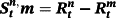
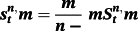
The relationship between the yield of a longer term n period, , and the yield of a shorter term m period, , under the rational expectation can simply be written as the following:

(1)

where k = n/m is an integer, φ_t denotes the information set available in time t, and θ is a constant parameter. E_t denotes the rational expectation conditional on information available at time t. Therefore, the n period interest rate is a constant, plus a simple average of the current and expected future m period rates up to k-1 periods in the future. The parameter θ reflects a term premium that is a predictable excess return on the k period bond over the one-period bond. The term premium is presumed to vary with k but is assumed to be constant through time.

Fama (1984) indicates that Equation 1 can be obtained from all discount bonds if one assumes that expected continuously compounded yields to maturity on all discount bonds are equal, up to a constant. It can be derived as linear approximation to any non-linear expectations theories of the term structure. If we focus our attention on the behaviour of the spread through time between the n period rate and the m period rate, the EH of the term structure implies that the spread is a constant time premium, plus an optimal forecast of changes in future interest rates. For instance, if n = 2 and n/m = 2, m = n–m. Equation 1 reduces to

(2)

After some algebra, Equation 2 can become

(3)

This expression reflects that the fact that under the EH, the current value of the spread should help to predict the value between the future spot rate and long-term rate. To be more precise, we can write the following equation:

(4)

where is the ex post realized rate at time t + m for the period n–m. In this case, n/m is not necessarily an integer. According to rational expectations (Muth, 1961), u_t + m is the forecast error at time t + m assuming to be orthogonal with the information available at time t. We test the null hypothesis of β = 1 to examine whether there is an unbiased predictor of future changes in interest rate when using any combinations of the spread. The Newey and West (1987) procedure is applied to get rid of the problem arising from overlapping data.

Using the Treasury rates with various combinations of n and m in the period between 1952 and 1971, Campbell and Shiller (1991) find that the coefficients are negative in most cases, indicating that the spread between long-term and short-term yields predicts an opposing movement of future interest rate. The results are apparently against the EH and have become a puzzle for researchers, hence stimulating further discussions.

Table 1 presents the estimates of the regression model using Equation 4 where the monthly U.S. zero-coupon bond yields for the period between March 1987 and December 2010 have been employed. 1 We find that the hypothesis of β = 1 is rejected for all cases at the conventional significance level, except for some cases in m = 12, indicating that the EH of the term structure is not held for most of the cases. Asymptotic standard errors, which have been corrected for heteroskedasticity and equation error overlap, in the manner of Newey and West (1987), almost show that the coefficients of β are insignificant, suggesting that the slope of the term structure fails to predict the change in interest rates, particularly for the short-term forecast horizon. For m = 12 and 24, the short end of the term structure shows a superior predictive ability for the movement of interest rates.

Equation 4 may be incorrectly estimated because the regression results do not consider possible structural breaks during the sample period. The Chow test rejects the null hypothesis of no structural break and detects a break in August 2007. It is well known that the subprimed crisis began in the United States and spread around the globe. Before that period, 10-year Treasury bond rate is greater than 3-month Treasury bill rate, but they become opposite after that period. At best, we shall use structural break model that may yield better estimates. However, the period after August 2007 contains only small sample (less than 3 years); the estimate using full sample without considering structural break model is not likely to alter our results.

By investigating the period between 1952 and 1987, Campbell and Shiller (1991) find an opposing direction when forecasting the yield changes of long-term discount bonds over the life of short-term discount bonds, which is referred to as a “term structure anomaly.” Table 1 shows that the anomaly has almost vanished during the latter period in comparison with the period studied by Campbell and Shiller (1991). However, the anomaly still remains on short forecast horizons (m = 3 and 6) and the long end of the term structure (n–m > 24). So far, previous works have related the term structure anomaly to the time-varying term premium (Jongen et al., 2011) or peso problems (Bekaert, Hodrick, & Marshall, 2001; Chen, Kuo, & Chiang, 2014; Jardet, 2008; Lewis, 1991). However, this study addresses it from the other angle. We proceed the decomposition in Equation 1, the term premium component and the expectation error component, and evaluate their contributions to the anomaly in the following section.

3 TERM PREMIA AND EXPECTATION ERROR

3.1 Decomposition of term structure anomaly

The results are in accordance with Campbell and Shiller (1991). We now turn our attention to the post Campbell–Shiller period and find that, although the spread provides a right direction of the prediction, support on the EH is still hard to achieve throughout the subsample. To study the cause, we provide a procedure to decompose the β coefficients in Equation 4.

First, let and . Then after rewriting Equation 4, we obtain Equation 5:

(5)

where

(6)

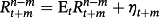where and η_t + m is the expectation error term, which assumes a random number under rational expectation. Then the left-hand side of Equation 5 can be specified as

(7)

where E_t is the expectation indication at time t for the rate at time t + m for the period n–m. In addition, we know that the term premium, is defined as the difference between the spread and expected future spot rate at time t for the period between n and m, 1 . Hence,

(8)

Inserting Equation 8 into Equation 7 yields

(9)

By substituting Equation 9 into Equation 6, we obtain

(10)

(11)

where

(12)

(13)

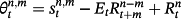
The subscript tp denotes the term premium, equal to where the subscript ee is the expectation error, defined as . Note that the beta decomposition is based on spreads rather than the forward premiums used by Froot (1989).

3.3 Decomposition of expectation errors

Table 3 reveals that expectation errors contain rational and irrational components. In this section, we attempt to split β_ee in Equation 13 to reflect these two components. Rational components result from the unknown factors at the time when the forecast is made, and irrational components are due to the difference between the true process of interest rate movement and estimates from market participants. The former should produce unsystematic error and is independent of past rates and the spread of long and short rates. Nevertheless, the latter one is more likely to generate systematic errors and has a persistent property. We demonstrate this relationship through some algebra. As assumed above, the expectation error is a linear combination of rational component (F) and irrational component (I). We express the expectation error as

(14)

where 0 < ω ≤ 1.The rational component may encompass macroeconomic surprises, the peso problem, 0 learning behaviour, or other rational factors. Macroeconomic surprises are measured as the biased estimation arising from incorrect prediction of macroeconomic variables. This issue will be discussed further below.

By replacing Equation 14 into β_ee in Equation 13, we get

(15)

hence,

(16)

where

(17)

(18)

Decomposing the β_ee into β_I and β_F permits us to examine the significance of the irrationality captured by β_I. As long as we declare the significance of β_I, the statement of irrationality naturally becomes valid. We show the evidence in the following section.

4 IRRATIONALITY AND EXPECTATION ERROR

One of the objectives of this study is to study whether irrationality during the post Campbell–Shiller period can explain the term structure anomaly. We found that term premia contributes more to the failure of the EH than the expectation error for the short end of the term structure, but for the long end of the term structure, expectation error dominates. To specify which part of the expectation errors is more critical in term structure anomaly and leads to a rejection of EH for the long end of the term structure, we proceed to explore the determinants of time-varying expectation errors.

As mentioned above, the expectation errors are decomposed into rational and irrational components. Three streams of previous literature explain the sources of rational factors. The first stream of rational variables includes the variables governed by peso problems (Bekaert et al., 2001; Evans, 1996; Jardet, 2008) and learning behaviour (Lewis, 1989). Peso problems arise from infrequent discrete shifts in economic determinants causing asset price behaviour to differ from conventional rational expectation. It is reasonable to assume that experience leads market participants to rationally predict future interest rates. When rare events occur, their expectations about future interest rates generate expectation errors. The learning behaviour of market participants also creates expectation errors because they gradually absorb and adjust their expectation when the rare events occur.

Second, expectation errors can arise from prediction of rates using equilibrium interest rate models, such as Vasicek (1977) or Cox, Ingersoll, and Ross (1985) models, which are formulated with assumptions of economic variables, and derive a process for short-term interest rates. Inconsistency between the assumptions behind these models, in regard to what economic variables evolve and the actual movement of the variables, could cause incorrect estimation of future interest rates. When these models are adopted for estimating future interest rates, systematic expectation errors between ex post realized rate and expected future interest rates may be generated.

The third stream of literature relates to incorrect estimation of macroeconomic variables where certain variables govern the interest rate changes. As pointed by Bartolini, Bertola, and Prati (2002); Benkert (2004); and Deuskar, Gupta, and Subrahmanyam (2008), default spread, inflation, money supply, and yield spread affect interest rate movements. Unexpected changes or shocks in inflation, for example, can create erroneous estimations in interest rates. Fama (2006) discusses the phenomenon of downward movement for U.S. 1-year interest rates for the period between 1981 and 2004, as the result of permanent shocks. Certainly, an unexpected change in interest rates may arise from the phenomenon of peso problem, the learning behaviour of market participant, incorrect model estimation, and so on.

Apart from rational variables, irrational components can impact expectation errors, for example, when investors trade fixed-income securities by extrapolating the trend or predict continuity of interest rates. Trend-chasing investors typically produce continuous errors across time, often resulting in persistently high number of correlated lags.

To obtain a suitable proxy for rational variables including peso problems, investor learning behaviour, and incorrect estimation of macroeconomic variables, we use the so-called macroeconomic surprises, defined as a vector of the unexpected relevant macroeconomic variables. There are three reasons that these surprise variables capture all rational variables. First, because macroeconomic variables are directly linked to interest rate movements, uncertain movements in these variables are bound to create an expectation error. In particular, uncertainty about economic variables is likely to disturb the probability distribution of interest rates that investors use to form their expectations when making financial decisions.

Second, information about the new stochastic process for interest rates is limited and/or may be revealed gradually, because agents learn about interest rate processes only from past information, and the ex post distribution may not agree with the ex ante distribution even based on rational expectations. With limited information available to agents, it is assumed that peso problems, learning behaviour, and incorrect estimation of economic variables are closely tied to the unexpected components of macroeconomic variables. In fact, unobserved regime changes or policy innovations can lead to surprises in macroeconomic fundamentals. Therefore, peso problems can be examined by testing their significance in relation to surprises resulting from macroeconomic variables.

Following Bartolini et al. (2002), Benkert (2004), and Deuskar et al. (2008), we use default spread, inflation, money supply, and yield spread as economic variables. Default spread (DEF) is obtained from the difference between 3-month LIBOR and Treasury bill rate, the so-called TED spread. This spread is often used as an indicator of market default in practice. Inflation (INF) affects the rate change in the way that higher inflation triggers higher nominal interest rates. Money supply (M2) is often used by central banks to control circulation of currency and inflation. This is done by changing interest rates. The yield spread (YIS), obtained from the difference between 5-year and 1-year rates, represents the market forecast of future interest rates.

Specifically, the ARIMA model is employed to estimate unpredictable (or unexpected) components from the time series of each economic variable. The estimated residuals for each variable and their corresponding standard deviations from the ARIMA model can be used to form the “surprise” series. The ARIMA model depicts the dynamics of a variable and explains its evolution based on its own lags and the lags of the other related variables. This feature is in accordance with a dynamic learning behaviour in that historical information is generally used to predict future interest rate movements. We therefore use the ARIMA model to remove serial correlated components, which do not impact expectation error, and to calculate residuals as macroeconomic surprises. First, each variable is differenced to account for nonstationarity. Second, based on the correlogram of each variable, the lag of the AR and/or MA component is determined and then the ARIMA model is run to generate a residual series for the surprise variable.

To measure the irrational variables, we follow Brown and Cliff (2004) and Baker and Wurgler (2006). Brown and Cliff (2004) provide a list of direct and indirect sources of sentiment proxies. The former is obtained from surveys, and the latter is derived from market trading activities. The direct sentiment proxies considered in this study are AAII, the Michigan consumer index, and the survey data from MarketVane. Another sentiment proxy is the monthly Baker and Wurgler Sentiment Index (Baker). Appendix B provides a description of these sentiment indices.

The indirect measures of sentiment proxies are mainly obtained from derivatives markets. Trading information in futures and options markets is considered as forward looking of market movement because market participants trade derivatives and risk their wealth based on their assessments of future price movement. First, put/call volume ratio (PCratio) obtained from Eurodollar options is considered as a bearish (bullish) indicator of Eurodollar futures (3-month Libor rate). Second, Commodities Futures Trading Commission (CFTC) reports the long/short volume for futures contracts traded in the United States. The net position in the 13-week Treasury bill on noncommercial traders is used as a proxy for institutional sentiment (INSTIT) and activity by small traders is used as a proxy for individual sentiment (INDIVD).

To remove nonsentiment-related component from each proxy, we follow Baker and Wurgler (2006) by constructing a common component, the first principal component from principal component analysis (PCA), from all variables. 1 By applying the PCA, we construct a composite sentiment index comprising the (a) AAII bearish percentage, (b) Michigan consumer index, (c) the bullish consensus for Eurodollar futures, (d) Baker and Wurgler Sentiment Index, (e) Eurodollar put/call volume ratio, (f) net long/short volume for noncommercial traders, and (g) net long/short volume for small traders.

Table 4 displays the regression results from time series of interest rate data for 3- and 6-month forecast horizons, whereas Table 5 shows those with 12- and 24-month forecast horizons. Note that each regression includes the AR(1) component to control for serial correlation in the expectation errors, which may boost the coefficient and affect subsequent inference of our results. As can be seen, all equations show various scales of significance for macroeconomic surprises and sentiment variables. The R² values are between 0.20 and 0.60, where the higher the forecast horizon the higher the value of R².

Default spread and yield spread surprises are significant for nearly all cases at the 1% level. Default spread is negatively related to time-varying expectation errors whereas yield spread is positively related. As we know, default spread is an acceptable measure of the aggregate liquidity variable as well as the default risk of constituent banks in U.S. dollar fixing. Incorrect estimation of this variable can affect the estimation of general interest rate level. However, yield spread is an indicator of economic conditions as well as the direction of expected future interest rates. Hence, an erroneous prediction of yield spread leads to invalid expectations about future interest rates, contributing to expectation errors.

The inflation and M2 surprises series generally follow a certain trend. Because money supply variable is strongly tied to inflation, our results show that they are not joint significantly related to expectation errors. Once the money supply surprise variable is significant, this variable absorbs the forecast power of inflation surprise, resulting in insignificance. Conversely, when the inflation surprise variable dominates, the money supply variable loses its influence. The argument is supported by the correlation ranging from −0.74 to −0.85.

Irrational variables proxied by selected sentiment variables show convincing results. First, the R² value on average increases by 2% when the equation includes sentiment variables (not reported). Particularly, long-term rates coupled with long-term forecast horizons tend to produce higher R² values than other cases. Second, the sentiment index appears to be significant for most cases including short-term forecast horizons in Table 4 and long-term forecast horizons (particularly 24 month) in Table 5. A negative coefficient indicates that a bullishness consensus in expected future rate spurs the expected future rate, producing negative expectation errors. The ex post realized rate is consequently less than the expected future rates. Conversely, a bearishness consensus may trigger a decline in the expected future rate, which causes the ex post realized rate to surpass the expected future rates and results in a positive expectation error.

Irrespective of forecast horizons, expectation errors for long-term securities appear to be governed more by investor sentiment than short-term securities, as evidenced the consistent significance of securities with 60- and 120-month maturities. One possible interpretation is that long-term securities prices are more sensitive to change in interest rates than short-term prices and hence are more likely to be affected by irrational investor sentiment. Another interpretation relates to Fama (2006) who indicates that swings of spot rates for short-term forecast horizons are driven by slow mean reversion, but spot rates for long-term forecast horizons are driven by permanent shocks to the long-term expected spot rate. As seen in Tables 4 and 5, even short- or long-term changes of spot rates are affected by several series of macroeconomic surprises. When surprises occur, irrational investor behaviour also affects expectation errors, leading to a predictive divergence from the slope of the term structure. Long-term securities, however, are more vulnerable to these shocks and are more closely related to investor behaviour.

5 CONCLUSIONS

Unbiased predictors of long and short rate spread have been rejected overwhelmingly by previous studies. Based on various maturities of U.S. Treasury yields and forecast horizons, Campbell and Shiller (1991) show that long–short rate spreads provide an opposing forecasts of spot rates. This phenomenon is referred to as a term structure anomaly or puzzle in this study. Prior works suggest that this anomaly is attributable to term premia, peso problems, or investor learning behaviour. Looking at the post Campbell–Shiller period of U.S. Treasury yields from 3 months to 10 years, and forecast horizons from 3 months to 2 years, the anomaly does not appear to be as serious as before, when focusing on short-term forecast horizons and the long end of the term structure.

This study provides new insight from Bulkley et al. (2015) explaining the term structure anomaly and the failure of the EH. We found that the failure of the EH for the short end of the term structure is driven mainly by term premia. However, for the long end of the term structure, time-varying expectation errors primarily cause the failure. Across forecast horizons, expectation error tends to dominate the failure of the EH. Consistent with Fama (2006), diverging forecasts to the future spot rate and the long–short rates are attributable not only to the presence of term premia but also to the macroeconomic surprises (shocks) across forecast horizons. This study especially points out the deterministic role of investor's irrational behaviour on the term structure anomaly during the post Campbell–Shiller period.

REFERENCES

- 1 The data used in this study are described in Appendix A.
- 1 The EH implies that the spread is a term premium, plus an optimal forecast of changes in future interest rate (Campbell & Shiller, 1991, p. 497).
- 2 Bulkley et al. (2015) use the rates obtained from term structure of interest rates as expected future rates to calculate expectation errors. Then they found the pattern of expectation errors conforming to specific behaviour biases.
- 0 Peso problems arise whenever the ex post frequencies of states within the sample differ substantially from their ex ante probabilities and where these deviations distort econometric inference (Evans, 1996). When a peso problem is present, the sample moments calculated from the available data do not coincide with the population moments that rational agents would have used when making their decisions.
- 1 To be consistent with other macroeconomic variables, each sentiment proxy is differenced and then PCA is implemented to extract the common component.
- -8 Please see the website of U.S. Federal Reserve website for the zero-coupon: http://www.federalreserve.gov/releases/h15/data.htm