Machine Learning-Based Clustering of Layer-Resolved fMRI Activation and Functional Connectivity Within the Primary Somatosensory Cortex in Nonhuman Primates
Funding: This work was supported by National Institutes of Health, NINDS-2R01NS078680.
ABSTRACT
Delineating the functional organization of mesoscale cortical columnar structure is essential for understanding brain function. We have previously demonstrated a high spatial correspondence between BOLD fMRI and LFP responses to tactile stimuli in the primary somatosensory cortex area 3b of nonhuman primates. This study aims to explore how 2D spatial profiles of the functional column vary across cortical layers (defined by three cortical depths) in both tactile stimulation and resting states using fMRI. At 9.4 T, we acquired submillimeter-resolution oblique fMRI data from cortical areas 3b and 1 of anesthetized squirrel monkeys and obtained fMRI signals from three cortical layers. In both areas 3b and 1, the tactile stimulus-evoked fMRI activation foci were fitted with point spread functions (PSFs), from which shape parameters, including full width at half maximum (FWHM), were derived. Seed-based resting-state fMRI data analysis was then performed to measure the spatial profiles of resting-state connectivity within and between areas 3b and 1. We found that the tactile-evoked fMRI response and local resting-state functional connectivity were elongated at the superficial layer, with the major axes oriented in lateral to medial (from digit 1 to digit 5) direction. This elongation was significantly reduced in the deeper (middle and bottom) layers. To assess the robustness of these spatial profiles in distinguishing cortical layers, shape parameters describing the spatial extents of activation and resting-state connectivity profiles were used to classify the layers via self-organizing maps (SOM). A minimal overall classification error (~13%) was achieved, effectively classifying the layers into two groups: the superficial layer exhibited distinct features from the two deeper layers in the rsfMRI data. Our results support distinct 2D spatial profiles for superficial versus deeper cortical layers and reveal similarities between stimulus-evoked and resting-state configurations.
1 Introduction
Functional magnetic resonance imaging (fMRI) of the human brain has been used to investigate fine-scale structures, such as the cortical columns (Yacoub et al. 2007; Yacoub, Harel, and Ugurbil 2008; Shmuel et al. 2010; Zimmermann et al. 2011; De Martino et al. 2015; Goncalves et al. 2015; Tootell and Nasr 2017). We previously demonstrated a high spatial correspondence between BOLD fMRI and LFP responses to tactile stimuli at the columnar level (single finger representation) in the primary somatosensory cortex area 3b in nonhuman primates (NHPs). Several studies have also explored how fMRI responses to stimulation vary across cortical depths (Chen et al. 2013; Herman et al. 2013; Baek et al. 2016; Guidi, Huber, and Lampe 2016; Guidi et al. 2016; Guidi et al. 2020), while others have reported layer-specific differences in stimulus-evoked fMRI activation (Koopmans, Barth, and Norris 2010; Polimeni et al. 2010; Goense, Merkle, and Logothetis 2012; Chen et al. 2013; Poplawsky and Kim 2014).
Estimates of resting-state functional connectivity, derived by measuring temporal correlations between low-frequency fluctuations of MRI BOLD signals between regions (Greicius et al. 2003; Weng et al. 2010; Chen et al. 2011; Wu et al. 2011; Bassett et al. 2012; Liemburg et al. 2012), also show layer-specific variations (Mishra et al. 2019; Heynckes et al. 2023; Yang et al. 2025) in the somatosensory cortex. Precise descriptions of the spatial extents of BOLD activation in fMRI, which depend on contributions from distributed neural activity and the associated metabolic/hemodynamic changes (Logothetis 2003; Saad et al. 2003; Huttunen, Grohn, and Penttonen 2008), therefore require fine-scale, layer-specific analysis for both stimulus and resting-state conditions.
Previous studies have demonstrated MRI field-dependent effects. For instance, the spatial specificity of the BOLD signal elicited by a small point stimulus in the primary visual cortex (V1) (Wu et al. 2011) was found to have 3.5 and 3.9 mm point spread function (PSF) measured using FWHM (full width at half maximum) at 1.5 and 3 T MRI fields, respectively (Engel, Glover, and Wandell 1997; Parkes et al. 2005). At higher MRI fields, the measured PSF within V1 in response to visual stimuli was less than 2 mm at 7 T (Shmuel et al. 2007). Similar quantification of the spatial extent of PSF was also reported in the primary visual cortex (V1) (Chaimow et al. 2018) and secondary visual area V2 (Fracasso, Dumoulin, and Petridou 2021), using the spatial organization of ocular dominance columns (ODCs). These studies characterized the spatial BOLD responses as circular in the visual cortex, with the region of interest confined to a single MRI slice sampling the entire cortical depth. However, they did not provide specific information on potential differences across cortical layers. A remaining question is whether the spatial profile of BOLD fMRI signals varies across cortical layers (defined by dividing cortical thickness into three depths). Addressing this question would offer insights into layer-specific functional organization features of the cortex as revealed by fMRI.
The estimated PSF parameters in the visual cortex, as reported in the studies mentioned above and in our previous work on area 3b in monkeys, measured responses in single slices without considering the potential vasculature and hemodynamic influences across cortical depth. However, several studies have suggested that fMRI responses to stimulation vary along cortical depth (Silva and Koretsky 2002; Lu et al. 2004; Harel et al. 2006; Zhao et al. 2006; Bissig and Berkowitz 2009; Koopmans, Barth, and Norris 2010; Polimeni et al. 2010; Chen et al. 2013; Herman et al. 2013; Baek et al. 2016; Guidi, Huber, and Lampe 2016; Guidi et al. 2016). This study aims to examine how the functional columnar structure, specifically the single-digit representation in the somatosensory cortex, varies across cortical layers by delineating the 2D spatial profiles of fMRI activation in response to the vibrotactile stimulus applied to a single finger's distal pad. We optimized the data acquisition protocol by increasing the spatial resolution along the cortical depth axis, enabling fMRI sampling from three cortical layers within the S1 cortex at different depths. We compared the spatial extents of stimulus-evoked fMRI activation and the local resting-state correlation profiles within and between cortical layers. Two measures of spatial extents—the axis ratio and the area enclosed by the PSF—were also compared between functionally related but distinct regions, area 3b and area 1, within the S1 cortex. To assess the robustness of these spatial profiles in distinguishing cortical layers, we implemented a data-driven self-organizing mapping (SOM) approach (Kohonen and Somervuo 2002) to classify the layers based on the PSF parameters. We found statistically significant interlayer differences across the cortical depth, based on PSF spatial features and connectivity measured by interlayer correlation. The SOM analysis classified different layers with approximately 87% accuracy based on these features.
2 Materials and Methods
2.1 Animal Preparation
Four adult male squirrel monkeys (Saimiri bolivians, average 3 years old) were included in this study. The animals were sedated with ketamine hydrochloride (10 mg/kg)/atropine (0.05 mg/kg), then anesthetized with isoflurane (0.5%–1.0%) delivered with an N2O:O2 (70:30) mixture for the duration of the imaging session. Isoflurane levels were maintained at approximately 0.9% during fMRI data acquisitions. The animals were artificially ventilated, and their heads were physically stabilized in an MR-compatible frame to minimize motion. Vital signals, including heart rate, respiratory pattern, core temperature, ETCO2, and pulse oximetry, were monitored and maintained at appropriate levels throughout the imaging session. All the procedures followed the NIH guidelines and were approved by the Institutional Animal Care and Use Committee (IACUC) at Vanderbilt University.
2.2 MRI Data Acquisition
MRI scans were performed with a 9.4 T, 21 cm bore Varian/Agilent Inova spectrometer (Varian Inc., Palo Alto, CA, USA) with a 3-cm diameter transmit-receive surface coil positioned over the central and lateral junction where primary somatosensory cortices (S1, including areas 3b and 1) are located. Nine 0.67-mm-thick T2-weighted oblique structural images (FOV: 35 mm, TR = 200 ms, TE = 16 ms, in-plane resolution of 68 × 68μm2) were acquired before fMRI data acquisition (Figure 1). Multiple runs of resting-state (15 runs) and stimulus-driven fMRI data (30 runs) were acquired using a multi-shot gradient echo planar imaging sequence with an in-plane resolution of 0.547 × 0.547 mm2 (two shots, TR = 1.5 s, TE = 16 ms) and the same slice thickness as the structural images. An innocuous 8 Hz vibrotactile stimulus (20 ms pulses duration)—a vertical indentation (0.34 mm displacement) of a rounded plastic probe (2 mm in diameter)—was delivered to individual distal finger pads (typically D2 or D3). The probe was mounted on a piezoceramic actuator (Noliac) controlled by a Grass Instruments stimulator, which regulated the timing of stimulus presentation. Vibrotactile Stimuli were presented in seven alternating 30s off/on blocks during each fMRI run. Resting-state fMRI runs (300 volumes) were typically acquired before stimulus fMRI runs (300 EPI volumes).

2.3 fMRI Data Preprocessing
All fMRI runs underwent motion and slice timing corrections. Six parameters of motion, along with temporal signals extracted from selected white matter voxels containing at least 70% of the cumulative variance (derived using principal components analysis), were considered nuisance parameters and regressed out using a general linear model without applying spatial smoothing. The RETROICOR method (Glover, Li, and Ress 2000) was used to reduce physiological noise in fMRI signals. Resting-state fMRI signals were band-pass filtered (Chebyshev type2 IIR filter, cut-off frequencies 0.01 and 0.1 Hz) prior to voxel-wise and pairwise correlation analyses. The fMRI data in individual subject space were co-registered to high-resolution anatomic images using FSL (FLIRT). A temporal signal-to-noise mask (tSNR > 10) was applied to eliminate non-brain voxels for both stimulus-driven activation and resting-state connectivity analyses.
2.4 Detection of Stimulus-Driven Activations
To localize stimulus-driven activation in areas 3b and 1 of the S1 cortex, we performed voxel-wise analyses of BOLD time courses using a generalized linear model (GLM, spm12). A GLM was fitted to each voxel time course for each run. The stimulus paradigm, convolved with a canonical hemodynamic response function, was used as a predictor to model stimulus-driven BOLD activation. Stimulus-activated voxels were defined as those showing statistically significant stimulus-related BOLD signal changes (t > 2, p < 0.05, FDR corrected). A minimum cluster size of two contiguous voxels was used as an additional criterion to identify the activated regions. BOLD time courses for voxels in each of the three layers, with peak t values in area 3b and area 1, were averaged across stimulus epochs (seven epochs per run). Voxels showing signal changes (t > 2) from 4 animals across a total of 30 runs were chosen to quantify the percentage BOLD signal changes. The signal was averaged over a six-second window before the onset of each stimulus cycle (four EPI data points) and used as the baseline to calculate percentage signal changes. A double gamma fitting of the mean signal, along with the standard error of the mean (SEM), was used to derive parameters describing the signals across cortical layers (depths).
2.5 Quantification of PSF Parameters of BOLD Signal in Stimulus and Resting State
In our previous work, we found that the patterns of vibrotactile stimulus-evoked activation were elliptical in shape in the finger representation in areas 3b and 1 (Shi et al. 2017) at a coarser level (2 mm slice thickness). In this study, we derived PSF parameters along both the major and minor axes to quantify the spatial distribution of the elliptical stimulus-evoked activation at a finer level, with the S1 cortex subdivided into three layers (0.67 mm thick). The FWHM along the major (long) and minor (short) axes was measured by applying a Gaussian fit to the 2-D cross-section map. For the resting-state fMRI connectivity analysis, we estimated the parameters of the local correlation profile by selecting the peak-activated voxels (peak t values) as seeds in both areas 3b and 1. Identical 2D spatial fitting was applied to estimate (1) the major and (2) minor axes, (3) the area enclosed by the FWHM contour, and (4) the ratio of major to minor axes of the PSF. Layer-specific comparisons of the four PSF parameters across the cortical depth were performed, and their statistical differences were evaluated using one-way ANOVA. The statistical significances of differences between measured parameters were quantified with p-values corrected for multiple comparisons.
2.6 Using Machine Learning to Classify Layers
We implemented SOMs (Kohonen and Somervuo 2002) to classify three layers according to their spatial profiles. SOM is an unsupervised learning technique that generates a low-dimensional representation of high-dimensional input data. This data-driven classification approach analyzed layer-specific PSF parameters, where SOM segregates a set of inputs into a user-defined number of clusters. We compared the performance of four variants of input data: (1) the major and minor axes only, (2) major and minor axes with axis ratio, (3) major and minor axes with the area enclosed at FWHM, and (4) a combination of all four parameters. In the absence of reliable activation in the deepest layer in stimulus conditions, we grouped the PSF parameters into two clusters.
Our previous work on layer-specific connectivity (Mishra et al. 2019; Yang et al. 2025) between area 3b and area 1 of the S1 cortex suggests statistically significant interlayer differences in resting-state correlations. We, therefore, also evaluated the correlation z-scores (Fisher's transformation) between the layers of areas 3b and 1, where the mean time course of each source (seed) ROI was correlated with voxels within the target ROI. Inter-ROI correlations between layers of areas 3b and 1 were measured in the resting state, and the resulting correlation patterns for each layer were used to classify layers with SOM. Three connectivity patterns associated with each sub-region (areas 3b or area 1), yielding nine (3 × 3) correlation measures in total, were segmented into 2–3 clusters using the machine learning algorithm. The classification accuracy in both stimulus and resting-state data was estimated by bootstrap analysis. Finally, layer classification using SOM—based on parameters describing (1) spatial extents of activation in stimulus data, (2) resting-state connectivity profiles, and (3) interlayer resting-state connectivity—were compared.
3 Results
3.1 Spatial Distribution Profile of BOLD Responses to Tactile Stimuli in Areas 3b and 1
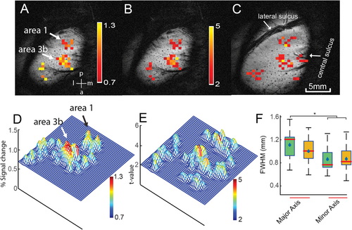
The responses to tactile stimuli applied to a distal finger pad were measured by estimating the FWHM along the major and minor axes. The ratio of the major and minor axes, along with the area enclosed by the fitted ellipse (using a 2D Gaussian fit) at half maximum, serves as an indicator of the spatial extent of the PSF along and across the digit representation. Figure 2A,B, show the percentage signal changes and t-maps overlaid on the anatomic images on the top slice (superficial layer), displaying activation patterns in areas 3b and 1 in response to stimuli presented to digit 2 (D2). Figure 2C shows the t-map on the middle slice, which has similar activation patterns in both areas. Figure 2E,F, present a 3D view of the activation patterns on the top layer, revealing the local spatial profile of activation. The BOLD responses in areas 3b and 1 appear as elongated ovals with the major axis oriented in the lateral-medial direction. The boxplot in Figure 2G shows the distribution of FWHM values along major and minor axes in the top and middle layers. The BOLD response, measured as FWHM along the major axis, is statistically significantly different from the minor axis in both the top and middle layers (p < 0.05, corrected for multiple comparisons) as determined by one-way ANOVA. Activation in the bottom layer was observed in only a few runs and was statistically insignificant in most cases. Consequently, the ROIs used for resting-state analyses in this layer (see below) were defined by extrapolating the spatial coordinates of the 2nd layer.
3.2 Layer-Specific Percentage Signal Changes in Response to Stimuli
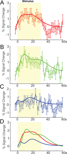
We evaluated the percentage signal changes in the peak-activated voxels in areas 3b and 1 relative to the baseline signal. Signal changes in area 3b across three consecutive layers (1–3) are shown in Figure 3A–C. A double gamma fit to the signal over seven epochs across eleven runs (n = 4) is depicted by the bold line from top to bottom layers, along with the mean and standard errors. Figure 3D illustrates the overall percentage signal change across the cortical depth, along with the double gamma fitting. The fitted curves reveal a significant drop in percentage signal in the deeper layer during the stimulus epoch. Although we did not detect activated voxels in the third bottom layer in all the animals at t > 2, the signal change in the extrapolated voxel in the bottom layer serves as a control, showing substantially lower signal change compared to the other two layers. The response to the stimulus is slightly faster in the superficial layer compared to the middle layer, though the peak activation is relatively larger in the middle layer.
3.3 Spatial Specificity of Resting-State Connectivity Patterns
After identifying the strongest stimulus activation foci (highest t values) in area 3b and area 1, we constructed ROI masks to evaluate the resting-state connectivity patterns (local correlation pattern) in the same animals (n = 4 animals, 15 runs). The FWHM along the major and minor axes, their ratio, and the area enclosed were measured (threshold: r = 0.5 for resting data). Figure 4A,C,E, show the resting-state connectivity patterns of the area 3b seed across three layers (top, middle, and bottom), overlaid on structural images. These resting-state correlation maps closely resemble the activation profiles observed under stimulus conditions (compare with Figure 2). When the seed ROI was switched to area 1, a similar local resting-state correlation profile was observed (Figure 4F). Figure 4B,D, show 3D connectivity profiles for the top and middle slices, respectively. Figure 4G displays an axial view of the contours describing the major and minor axes of the fitted ellipse at half maximum, characterizing the PSF.
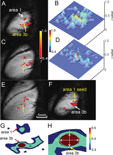
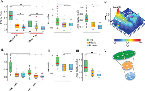
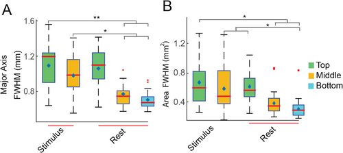
Figure 5AI–III present boxplots showing the distribution of four resting-state local correlation parameters measured in area 3b. A group-level comparison of the major and minor axes across the cortical depth (top to bottom) indicates that the major axis in the top layer is significantly larger than its minor axis, and the major and minor axes of the middle and bottom layers (p < 0.005, corrected for multiple comparisons, Figure 5AI). Significant differences were also observed between the minor axes of the top and bottom layers of area 3b, differences that were not prominent in stimulus-driven activations. When comparing axis ratio and area, significant differences (p < 0.005) were found between the top and bottom two layers (Figure 5AII&III). Similar differences were observed in area 1 (Figure 5BI–III). No differences were found between the corresponding parameters of each cortical layer between areas 3b and 1. The minor axis did not show comparable significance in differences to the major axis in area 1 (Figure BI). A 3D surface and cross-sectional view illustrate the variation of resting-state connectivity profiles along the cortical layers in area 3b (Figure 5A,BIV). Table 1 shows the FWHM along the major and minor axes measured across cortical depth for both stimulus and resting-state data. When comparing parameters derived from stimulus-driven and resting-state conditions, the major axes in both the top and middle layers during stimulus conditions were significantly larger than the major axes in the middle and bottom layers during the resting state. Similar differences were observed while comparing the area of the PSF at half maximum (Figure 6A,B). In summary, stimulus-evoked BOLD responses in areas 3b and 1 were elliptical, with the major axis oriented in the lateral-medial direction, while the resting-state correlation profile in the top layer was slightly elongated.
| Layer | Major axis (mm) | Minor axis (mm) | |
|---|---|---|---|
| Stimulus | Top | 1.07 (±0.26) | 0.81 (±0.23) |
| Middle | 0.96 (±0.24) | 0.81 (±0.23) | |
| Resting | Top | 0.99 (±0.25) | 0.75 (±0.15) |
| Middle | 0.72 (±0.14) | 0.67 (±0.13) | |
| Bottom | 0.69 (±0.08) | 0.63 (±0.07) |
3.4 Classification of Layers Using Machine Learning
Based on differences in PSF features across layers, we implemented SOM to classify the three layers using four input parameters (major, minor axis, axis ratio, and area). Bootstrapping was performed to improve variance estimates by resampling the input to the SOM 500 times from the entire pool of parameters associated with the layers (N = 4, 30 runs). The success of layer classification was quantified as a percentage. Table 2 shows the mean and standard error of classification success rates for both stimulus and resting-state data. Feature selection has a substantial impact on algorithm performance. Notably, a three-feature combination—major axis, minor axis, and the area enclosed at FWHM—resulted in significantly higher classification accuracy (~87%) in resting-state data, particularly for distinguishing the top (layer 1) and bottom (layer 3) layers. Comparable accuracy (~86%) was observed when the axis ratio was included. Accuracy decreased to approximately 81% considering layers 1 and 2 in the resting state. For stimulus-driven data, classification accuracy was lower (~75%) when all FWHM parameters were included.
| SOM % accuracy (PSF) | |||
|---|---|---|---|
| Parameters | Stimulus | Resting | Resting |
| Layer 1 ~ 2 | Layer 1 ~ 2 | Layer 1 ~ 3 | |
| Major & minor axis | 68.47 (±11.3) | 78.75 (±5.3) | 86.07 (±4.9) |
| Major, minor axis, and area | 70.42 (±10.2) | 80.93 (±5.6) | 86.93 (±4.4) |
| Major, minor axis, and axis ratio | 69.47 (±9.8) | 68.79 (±5.8) | 73.12 (±5.9) |
| Major, minor axis area, and axis ratio | 75.04 (±9.7) | 73.34 (±6.2) | 77.81 (±5.9) |
3.5 Classification Based on Interlayer Connectivity Between Area 3b and Area 1 in the Resting State
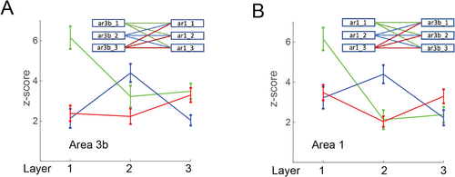
Layer-specific inter-ROI correlations between areas 3b and 1 were classified using SOM. Fisher z-score of nine measures for each run was used to generate nine connectivity patterns, as shown in Figure 7. The line plots show the corresponding connectivity patterns (correlation (z-score) between area 3b and area 1). We segmented layer-specific connectivity patterns and classified layer pairs into two groups, examining four combinations of layer pairs: layers 1–2, 1–3, 2–3, and 1 ~ (2 + 3). These combinations were tested to estimate and compare the segmentation accuracy (Table 3). The peak classification accuracy for layer pairs was approximately 79% when connectivity patterns between layers 1 and 3 were input to the SOM. Classification accuracy for layers 2 and 3 were considerably lower compared to other combinations. This reduction in accuracy may be attributed to the similarity in connectivity patterns between these layers. The classification performance of SOM depends on shape parameters under three conditions: (1) stimulus, (2) resting state, and (3) interlayer resting-state connectivity. Our results indicate that SOM is most efficient in classifying the superficial and deeper layers (1 ~ 3 and 1 ~ 2) in the resting state when the major axis, minor axis, and area enclosed at FWHM are used as input parameters.
| SOM % accuracy (RSFC) | |
|---|---|
| Layer | Area3b-area1 |
| 1 ~ 2 | 72.49 (±13.2) |
| 1 ~ 3 | 78.31 (±13.5) |
| 2 ~ 3 | 58.87 (±12.4) |
| 1 ~ 2 + 3 | 65.57 (±19.1) |
4 Discussion and Conclusion
4.1 Mesoscale High Spatial Correspondence Between Cortical Layers Within and Between Cortical Areas
Interpreting cortical layer-resolved fMRI data requires caution, as BOLD signals are indirect measures of neural activity and are influenced by vascular features. Cortical depth-dependent differences in neural activity and neurovascular coupling affect measurements of stimulus-evoked BOLD changes (Polimeni et al. 2010; Patel et al. 2015; Goense, Bohraus, and Logothetis 2016), but their influence on estimates of resting-state functional connectivity remains unclear. Our previous studies (Shi et al. 2017) showed that the spatial extents of stimulus-evoked activation within the somatosensory cortex (areas 3b and 1), produced by single-digit stimuli, are anisotropic, with the major axis aligning in the lateral-medial direction (along the digit tip-to-tip representation line). The somatosensory cortex in squirrel monkeys is approximately 2 mm thick, and we have previously reported interlayer and inter-areal connectivity differences (Mishra et al. 2019; Yang et al. 2025). To accurately quantify the spatial profiles of different cortical layers within and between areas 3b and 1, we optimized the fMRI data acquisition with oblique imaging planes that separate the three cortical layers.
In this study, we found that the PSF of stimulus-evoked activation was comparable to that of local resting-state correlation profiles, suggesting that the neurons that are responsive to natural tactile finger stimulation also exhibit synchronized fMRI BOLD signal fluctuation within areas 3b and 1 across cortical layers at the mesoscale (~ 500 micros). This finding extends our previous observation of high spatial correspondence between stimulus-evoked and rest-state BOLD signals and demonstrates this high correspondence across cortical layers.
To evaluate the consistency of spatial profiles revealed by PSF and to examine systematic differences between conditions (task versus rest) and cortical layers, we used a data-driven approach to classify cortical layers in areas 3b and 1. This classification was based on quantitative measures of PSF spatial profiles of BOLD responses and local connectivity patterns across the cortical depth. Our results showed that the choice of parameterized input vectors for the SOM algorithm affected the classification accuracy, which also differed between stimulus and resting states. Fine-tuning these parameters with additional data and higher resolution may improve layer classification accuracy in future studies.
4.2 PSF Shape Similarity and Classification Accuracy in Stimulus and Resting States
Spatial profiles theoretically reflect underlying neuronal activity and are influenced by neurovascular coupling. Interestingly, the shape similarity between PSF parameters in stimulus and resting-state correlation was comparable in terms of axis length, activation area, area of correlation profile, and axis ratio for each layer. We observed significant differences in area, axis ratio, and major axis across both conditions, with these differences being more pronounced in the resting state than in the stimulus condition. Greater variations in resting-state correlation parameters for both major and minor axes were also observed in comparison to the stimulus data.
Furthermore, PSF parameters in the resting state showed larger differences in area and axis ratio between superficial and deeper layers. In most animals, activation foci in the bottom under stimulus conditions could not be reliably identified, which prevented a one-to-one comparison between stimulus and resting-state parameters. Nevertheless, classification accuracy for distinguishing superficial (layer 1) and deeper (layer 3) layers in the resting state surpassed that of stimulus and layer-specific connectivity data. Similar classification accuracy was achieved when interlayer correlation z-scores (area 3b vs. area 1) in the resting state were used, indicating that the interlayer PSF identified by spatial profile analyses was consistent and reproducible.
4.3 Motivation Behind Using AI-Based Machine Learning Classification
Statistically significant interlayer differences in PSF parameters, particularly in the resting state and between stimulus ON/OFF conditions, motivated us to classify the layers using machine learning techniques with SOM. Bootstrapping, which involved random sampling with replacement, confirmed the SOM results, even with a moderate dataset of input parameters. Unlike conventional neural networks, SOM operates in an unsupervised manner and does not require a target vector for training. The modified SOM, also known as a self-organizing feature map (SOFM), used in this study, learns both the distribution and topology of the input vectors (Heskes 2001; Kohonen and Somervuo 2002). Our findings demonstrated the effectiveness of this approach, providing unbiased results that support the spatial profile differences between states and across layers at the mesoscale in the monkey cortex.
4.4 Vascular Influence on fMRI BOLD Signals Across Cortical Layers
The influence of large surface vessels on BOLD signals is well-documented. We recently reported that vascular structures influence fMRI BOLD signals differently across different cortical layers in area 3b of the cortex (Yang et al. 2025). Similar observations have been made in other systems. For example, the spatial profile of BOLD signals in the human visual cortex (Engel, Glover, and Wandell 1997; Parkes et al. 2005; Chaimow et al. 2018) has been shown to be influenced by the cerebrovascular organization. In this study, both the BOLD and LFP responses in areas 3b and 1 of the S1 cortex exhibited an elliptical shape, with the major axis oriented in the lateral-to-medial direction, corresponding to digit tip-to-tip representation (Chen et al. 2011; Shi et al. 2017).
Although it is known that BOLD signals in the superficial layer of the cortex are more influenced by large vessels, the elongated stimulus-evoked and resting-state spatial profiles along the digit tip-to-tip direction support a strong underlying neurophysiological basis. We expect that blood vessels influence BOLD signals in a non-directional manner, potentially yielding circular PSF parameters. The observed trend of reduced major axis in deeper cortical layers may indeed reflect distinct neuron composition and functionality differences across cortical layers. In summary, the distinct spatial profiles observed across cortical layers offer novel insights into the functional organization of the primate cortex at the mesoscale columnar level and provide new metrics to assess brain pathology in various disorders.
Acknowledgments
We would like to thank Chaohui Tang for her assistance with data collection and animal care.
Conflicts of Interest
The authors declare no conflicts of interest.
Open Research
Data Availability Statement
The codes and supporting documents are available in the public repository https://github.com/arimishra/repositoryHBM. Sample data will be provided upon request.


