Strategies for Developing Prediction Models From Genome-Wide Association Studies
Abstract
Genome-wide association studies (GWASs) have identified hundreds of single nucleotide polymorphisms (SNPs) associated with complex human diseases. However, risk prediction models based on them have limited discriminatory accuracy. It has been suggested that including many such SNPs can improve predictive performance. Here, we studied various aspects of model building to improve discriminatory accuracy, as measured by the area under the receiver operating characteristic curve (AUC), including: (1) How well does a one-phase procedure that selects SNPs and estimates odds ratios on the same data perform? (2) How should training data be allocated between SNP selection (Phase 1) and estimation (Phase 2) in a two-phase procedure? (3) Should SNP selection be based on P-value thresholding or ranking P-values? (4) How many SNPs should be selected? and (5) Is multivariate estimation preferred to univariate estimation in the presence of linkage disequilibrium (LD)? We used realistic estimates of the distributions of genetic effect sizes, allele frequencies, and LD patterns based on GWAS data for Crohn's disease and prostate cancer. Theory and simulations were used to estimate AUC. Empirical risk models based on 10,000 cases and controls had considerably lower AUC than theoretically achievable. The most critical aspect of prediction model building was initial SNP selection. The single-phase procedure achieved higher AUC than the two-phase procedure. Multivariate estimation did not perform as well as univariate (marginal) estimation. For complex diseases and samples of 10,000 or fewer cases and controls, one should limit the number of SNPs to tens or hundreds.
Introduction
Case-control genome-wide association studies (GWASs) for complex diseases have identified many single nucleotide polymorphisms (SNPs) that are associated with disease. However, risk models based on such SNPs have had only modest discriminatory accuracy as measured by the area under the receiver operating characteristic curve (AUC) (e.g. Jostins and Barrett [2011]). Two lines of evidence suggest that SNPs could provide much more predictive information, if only one could tap into the “missing heritability” suggested by phenotypic familial correlations. Purcell et al. [2009] and Stahl et al. [2012] showed that risk scores based on large numbers of SNPs could explain more heritability than those based on a small number of rigorously confirmed SNPs. Studies of correlations in GWAS data showed that all SNPs together account for much more heritability than the rigorously validated SNPs [Lee et al., 2011; Yang et al., 2010].
However, it is not possible to take advantage of this potential information to build discriminating risk models unless the sample size of the GWAS data for model building is large enough. Wray et al. [2007] used information on genetic architecture to conclude that half the heritability could be captured with 10,000 cases and controls, whereas Chatterjee et al. [2013] found that hundreds of thousands were needed for complex diseases. Even if the largest GWAS to date were tripled in size, the foreseeable AUC values based on the additional SNPs for many cancers would remain modest [Park et al., 2012], because most of the SNPs with the largest odds ratios have already been detected.
Feasible sample sizes are more modest for many complex diseases. Therefore we study model-building for sample sizes  ,
,  ,
,  and
and  , based on distributions of log odds ratios per allele developed for Crohn's disease and prostate cancer. We show that these distributions are consistent with heritability estimates on the liability scale [Chatterjee et al., 2013; Lee et al., 2011] and use them to investigate a number of facets of model-building. These include: (1) How well does a one-phase procedure that uses all the data to select SNPs and to estimate their effects perform, compared to a two-phase procedure that eliminates bias from the “winner's curse” [Zöllner and Pritchard, 2007] by selecting SNPs in Phase 1 and estimating effects from independent Phase 2 data? (2) What proportion of the data should be allocated to Phase 1 in the two-phase procedure? (3) Should one select SNPs by using a P-value threshold or by ranking P-values? (4) How many SNPs should be selected? (5) Does univariate or multivariate estimation perform better? (6) Should one filter out highly correlated SNPs? and 7) Do findings for AUC also hold for the probability of correct classification [Liu et al., 2012]? Unlike most previous work, we evaluate these strategies both in the presence and absence of linkage disequilibrium (LD). We also compare our results for Crohn's disease with those of Kooperberg et al. [2010], who used more complex modeling strategies on the same data.
Risk Model and Two-Phase Procedure
Risk Model
 denote the disease status of subject j (
 or 1), and let
  be the number of minor alleles for SNP i,
  for subject j, with minor allele frequency (MAF)
  . The vector of all SNP genotypes for subject j is
  . We let the first M of the N SNPs be truly disease associated, and assumed that the disease risk in the source population is given by
 (1)
(1) , μ is the intercept in the source population and
  is the log odds ratio for SNP i. The SNPs in 1 can also be in LD with themselves or with other SNPs.
Development (Phases 1 and 2) and Validation of Risk Model
In Phase k, there are  cases and
  controls,
  . The training data for Phases 1 and 2 consist of
  cases and n controls. The proportion
  and
and  are allocated to Phases 1 and 2, respectively. We use the term “training Data” to distinguish the “n” cases and controls used to build risk models from the independent validation data. We varied λ and other parameters to maximize the AUC, which is estimated with independent nontraining data.
Phase 1: SNP Selection
 (2)
(2) and the corresponding Wald statistic,
  for
for  . For all nondisease-associated SNPs, the asymptotic distribution of
  is a central
  distribution, and for disease-associated SNPs,
  a noncentral
  distribution, where the noncentrality parameter depends on
  , on the MAF
  , and on the sample size n1 [Gail et al., 2008]. Required variances are in Appendix A.1.1. We also computed
  , where
  is the
  quantile of a central
  distribution.
We selected disease-associated SNPs based either on P-value thresholding or on ranking of P-values. For P-value thresholding, we selected the ith SNP if its P-value was less than a prespecified cut-off. With ranking, all SNPs corresponding to the smallest T P-values were selected [Gail et al., 2008]. With P-value thresholding, a variable number,  , of SNPs were selected, while ranking led to exactly
  selected SNPs.
Phase 2: Estimating Log Odds Ratios
 index the SNPs selected in Phase 1. We used independent Phase 2 data to estimate
  for the
  SNPs and fitted both multivariate logistic regression,
 (3)
(3) (4)
(4) . In the presence of LD, we excluded some highly correlated SNPs (Appendix B).
Model Validation: Score Computation and AUC Estimation
 (5)
(5) . We estimated AUC nonparametrically from the Mann–Whitney statistic. In independent validation data, we always set n3 = 400 cases and n3 = 400 controls, which results in
  = 0.0004 (Appendix A.1.2).
Simulating Case-Control Data to Estimate the AUC
Simulating a Source Population With Joint SNP Genotypes in the Presence of LD
To generate case-control data, we applied model 1 to a source population of individuals with joint SNP genotypes. To simulate that source population, we used the distribution of genotypes among controls from the Welcome Trust Case Control Consortium (WTCCC) study of Crohn's disease after imputation of missing SNP genotypes [Kooperberg et al., 2010].
Dr. Kooperberg kindly provided us the data on 2,938 controls, each with complete genotypes on 333,187 SNPs. The corresponding MAF distribution had mean 0.260 and standard deviation 0.13. The MAF for each SNP was regarded as fixed and equal to that in the 2,938 controls. To preserve LD, we generated a subject from the source population by independently sampling the joint SNP genotypes for each of the 22 pairs of autosomes. The joint SNP genotypes for each pair of autosomes were sampled with replacement from its set of 2,938 joint SNP genotypes in controls.
Distributions of Log Odds Ratios for Truly Disease-Associated SNPs
To use model 1, we needed to assign  values to the disease-associated SNPs; other SNPs had
  . Under LD, we assigned disease-associated SNPs at random to the locations
  . We summed only over those disease-associated SNPs in equation 1. We used unpublished parameter estimates provided by Dr. Ju-Hyun Park (personal communication) for realistic distributions of
  derived from data used in Figure 2 of Park et al. [2011]. For Crohn's disease, Dr. Park provided a range ( − 0.058, 0.058) within which nonnull
  cannot be detected (power less than 1%) by the largest available GWAS datasets; SNPs are said to be “unobservable” in this interval. The distribution of the observed
  was well fitted by a two-component normal mixture
  , where
  ,
,  , and
, and  . Dr. Park provided these variance formulas, conditional on minor allele frequency, from data in Park et al. [2011]. To allow for the possibility that there are more SNPs in the unobservable range than implied by the two component mixture, we also considered a model that includes a third normal component in the unobservable range with mixture probability
  . The resulting mixed density is
  where now
  and
and  , and
, and  was chosen to assure that most (99.7%) of the mass of the third component was in the unobservable range. Supplementary Fig. S1 of the Appendix shows the marginal densities of
  after averaging over
  .
.
Park et al. [2010] estimated the number of disease-associated SNPs, M0, that will be found in observable ranges in future large GWAS. The probability  that a disease-associated SNP is in the observable range corresponds to the integral of the density outside the vertical lines in Supplementary Fig. S1. Thus the total number of disease-associated SNPs, M, can be estimated from
  . To compute
  and hence M, we averaged the conditional probabilities given
  over 106 random draws of
  .
.
Analogous methods and results are given for prostate cancer in Appendix C and Supplementary Fig. S1 in the Appendix.
The distributions of  and
and  together with M0 and π0, determine the true number of disease-associated SNPs, M, and
  , as well as the maximal achievable AUC (Section on Estimating the AUC under Linkage Equilibrium). The quantity σ2 determines the heritability on the liability scale,
  , and other properties(Appendices A and E and Supplementary Table S1 in the Appendix).
Estimating AUC Under LD From the Two-Phase Procedure
Having computed M, we assigned the disease-producing SNPs with their corresponding  to random loci to create a genotype structure (
 ), where only M of the
  are nonzero. We preserved this genotype structure in simulating the cases and controls for Phases 1, 2 and independent validation data. An individual with joint genotypes was sampled from the source population (Section on Simulating a Source Population with Joint SNP Genotypes), and a Bernoulli outcome with disease probability given by equation 1 was generated. The intercept in equation 1 was chosen such that the probability of disease was 0.01 in the source population. This process was repeated until
  cases and
  controls were identified.
In Phase 1, we used  cases and n1 controls to compute P-values from marginal logistic regression models 2, and we selected all SNPs with P-values smaller than a set threshold. Our algorithm to remove SNPs in very high LD is in Appendix B.
Estimation in Phase 2 was based on n2 cases and n2 controls. The AUC was estimated based on scores 5 computed for each of the 400 cases and 400 controls in independent validation data (Section on Development (Phases 1 and 2) and Validation of Risk Model). The simulation flowchart is shown in Supplementary Figs. S2 and S3. To maximize the AUC for given set of case-control data, we estimated the AUC over a grid of values of (P-value threshold, λ) or (T, λ) and chose the largest AUC estimate. The distribution of the maximum AUC was estimated from 20 such estimates from 20 independently sampled genotype structures,( ). To estimate the maximum theoretically achievable AUC, we replaced
  by the true values
  and used only the disease-associated loci in computing the score.
This simulation method can also be used to estimate AUC under linkage equilibrium, but we used a faster analytic method under linkage equilibrium (next section).
Estimating the AUC Under Linkage Equilibrium (Independence) for a Rare Disease
For rare diseases and linkage equilibrium, Gail et al. [2008] showed that conditional on ( ), SNP genotypes are independent in cases and controls if they are independent in the source population, and they gave the conditional genotype distribution for a SNP with given
  and
and  , both for cases and controls. Thus, the joint SNP genotype for each case or control could be obtained by drawing each SNP genotype independently, conditional on (
 ). With linkage equilibrium, there is no need to remove correlated SNPs and one can use simulations as in the previous section to estimate AUC. However, we computed AUC by faster methods, based on asymptotic theory in Gail et al. [2008] instead. In unreported numerical studies, we showed that these faster methods yielded results in agreement with the simulation methods in the previous section.
 while the remainder have
  , as in equation 1. Let
  if SNP i is selected in Phase 1 and 0 otherwise. We obtained Phase 2 estimates for the selected SNPs by drawing
  from a normal
  distribution for disease-associated SNPs and from
  for other SNPs, where
  depends on n2,
  and
and  , and
, and  depends on n2 and
  (Appendix A.1.1). Let
  correspond to the effects for selected disease-associated SNPs and
  the effects for all the other selected SNPs. In this notation the score for a person with genotypes
  is
is
 (6)
(6) , for large N and independent, bounded
  , the score is approximately normally distributed in cases and controls (Liapunov central limit theorem). The conditional moments of S in controls (S0) and cases (S1) are:
 (7)
(7) (8)
(8) and
and  from the retrospective distribution of genotypes [Gail et al., 2008].
 , the AUC can be expressed in terms of the cumulative normal distribution function, and the unconditional AUC can be computed by averaging the conditional AUC over
  and
and  as
as
 (9)
(9) is the joint probability mass function of the
  .
. , because the
  are independent Bernoulli variates with parameters
 (10)
(10) has a noncentral
  distribution with noncentrality parameter
  . Here
  is computed like
  in Appendix A.1.1, but with n1 replacing n2. For non-disease-associated SNPs,
  . When SNPs are selected by ranking,
  can not be computed explicitly. Both for thresholding and ranking, we thus used a Monte Carlo integration algorithm to evaluate equation 9. The flowchart of the simulation procedure is in Supplementary Fig. S3, and the algorithm is in Appendix A.1.4.
To find the combination of (P-value threshold, λ) or (T, λ) that approximately maximized the AUC, we evaluated equation 9 over a grid of values of (P-value threshold, λ) or (T, λ). Independent Monte Carlo integrations were performed for each point on the grid and the point yielding the largest AUC value was determined. This process was repeated for 20 independently sampled genotype structures ( ) to learn about the distribution of the maximum AUC,
  , and corresponding grid point.
To estimate the maximum theoretically achievable AUC, we used the true values ( ) to compute the mean and variance of the theoretically optimal score among cases, (
 ,
,  ), and among controls, (
 ,
,  ). The corresponding theoretically maximum AUC,
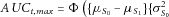
 .
.  was estimated as the average of 20 such estimates from 20 independent genotype structures (
 ).
).
Single-Phase Model
In the single-phase model, we used all the training data both for the selection of SNPs and for estimation of effect sizes. Under LD we simulated genotype data as in the Section on Simulating a Source Population with  . We did not estimate
  in Phase 2, but instead used
  for SNP selection and to estimate AUC in independent validation data. Correlated SNPs were eliminated as in Appendix B. Under linkage equilibrium, instead of sampling the selection indicator
  directly, we drew
  from
from  for all training data, where
  is a function of n1 and
  . We calculated Wald statistics
  for
for  , drew
  from
from  , and
, and  for
for  . We set
  if
if  and 0 otherwise. In the validation data, we used
  from Phase 1 to compute the AUC using formula 9 with
  and
and  .
.
Simulation Results
Rare Disease and Linkage Equilibrium
We begin with the case of linkage equilibrium to facilitate comparisons under LD in the next section. Park et al. [2010] estimated M0 = 142 observable SNPs for Crohn's disease and somewhat more than 66 for prostate cancer. Both estimates have wide ranges of uncertainty. For each disease, we investigated  1,000 and 3,000 and 10,000 and 100,000, the choice of SNP selection criterion (P-value thresholding vs. ranking),
  or 0.6, and various choices of M0 to determine which of these factors affected
  . To find
  , we searched over the set of P-value thresholds:
 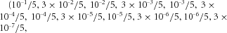 and
and  . In figures, we index these thresholds on the log base 10 scale as
  P-values
 . For example the P-value threshold
  has index approximately 5.5. For ranking, we chose T from the set (1, 10, 30, 100, 200, 300, 1,000, 3,000). Note, for example, that if
  and all
  , the expected number of SNPs selected is 30 for P-value threshold
  . In either case, the allocation ratio λ was chosen from the set (0.4, 0.5, 0.6, 0.7, 0.8, 0.85, 0.9, 0.95). Results in corresponding figures and tables are the means (with standard deviations) over 20 independent realizations of genotype structure (
 ,
,  ).
).
Figure 1 shows how  varies with λ for various values of P-value threshold or T for Crohn's disease with
  and
and  and for a single genotype structure (
 ). For P-value thresholding,
  is found for P-index = 3.5 (or P-threshold
  ) at
) at  . It is apparent that the majority of the training data should be allocated to SNP selection (Phase 1). Less stringent thresholds or more stringent thresholds yielded lower AUC. SNP selection based on ranking yielded similar results, with
  at T=30 and
  .
.

 or for different numbers of top-ranked SNPs, T, for one realization of genetic structure (
 ) under linkage equilibrium. For Crohn's disease,
  ,
,  ,
,  , and
, and  . For prostate cancer,
  ,
,  ,
,  , and
, and  .
.Table 1 presents averages over 20 realizations of ( ) for Crohn's disease with P-value thresholding. The case
  and
and  corresponds to a heritability
  ranging from 0.094 for disease probability 0.001 to 0.279 for disease probability 0.05 (Supplementary Table S1). For this case, there were on average
  truly disease-associated SNPs. Of these,
  were selected in Phase 1 with
  , and of those selected,
  were truly disease-associated SNPs on average. In 12 of the 20 genotype structures studied, the maximum occurred at (P-threshold =
  ,
,  ), and in eight instances at (P-threshold =
  ,
,  ). The
  increased from 0.591 for
  to 0.664 for
  to 0.740 for
  (Supplementary Table S2). Thus
  increased strongly with n. Larger samples led to the selection of more truly disease-associated SNPs on average (
 for
for  and 774.1 for
  (Supplementary Table S2)). The
  = 0.740 for
  is very near the theoretical maximum,
  = 0.756 (Supplementary Table S1). Similar results were found for
  , which more than doubled the number of disease-associated SNPs, M, and increased the heritability by about 30% (Supplementary Table S1) but had little impact on the numbers of disease-associated SNPs selected nor on AUC (Table 1). Most of the additional disease-associated SNPs were too small to detect with
  , although the
  increased to 0.782 (Supplementary Table S1). With
  ,
,  = 0.753 (Supplementary Table S2). Using ranking instead of P-value thresholding yielded very similar results(Supplementary Tables S3 and S4).
 ), under linkage equilibrium. Maximization is over
  and P-value threshold. Parameters that were varied include
  , M0 and π0. Total number of SNPs was
  . M0 denotes the number of disease SNPs in the observable range; M denotes the total number of disease SNPs;
  denotes the average number of SNPs selected and
  denotes the average number of truly disease-associated SNPs selected.
  denotes the number of times one combination of (λ, P-value) maximizes the AUC in 20 independent replications of the entire experiment
 |
 |
||||||||
| Two-phase model | Single-phase model | Two-Phase Model | Single-Phase Model | ||||||
|---|---|---|---|---|---|---|---|---|---|
| M0 |  |
 |
 |
 |
 |
 |
 |
 |
|
| 100 | AUC (sd) | 0.560(0.016) | 0.555(0.014) | 0.570(0.017) | 0.564(0.014) | 0.616(0.014) | 0.612(0.013) | 0.622(0.013) | 0.618(0.013) |
| M (sd) | 770.1 (0.605) | 1,866.2 (1.20) | 770.1 (0.605) | 1,866.2 (1.20) | 770.1(0.604) | 1,866.2(1.20) | 770.1 (0.605) | 1,866.2 (1.20) | |
 (sd) (sd) |
10.9 (2.78) | 11.2 (4.42) | 7.46 (1.89) | 6.75 (2.58) | 38.0(9.74) | 40.1(10.8) | 27.7(3.23) | 27.6(3.64) | |
 (sd) (sd) |
4.97 (1.58) | 4.61 (1.41) | 5.65 (1.71) | 4.99 (1.64) | 24.7(3.31) | 25.5(5.12) | 25.4(2.96) | 25.6(3.64) | |
 (λ, p) (λ, p) |
17  |
16  |
17  |
12  |
10  |
8  |
19  |
20  |
|
3  |
3  |
3  |
7  |
6  |
8  |
1  |
- | ||
| - | 1  |
- | 1  |
4  |
4  |
- | - | ||
| 200 | AUC (sd) | 0.591(0.013) | 0.591(0.017) | 0.604(0.017) | 0.591(0.017) | 0.664(0.012) | 0.662(0.016) | 0.672(0.012) | 0.670(0.016) |
| M (sd) | 1,539.6(1.10) | 3,732.0(2.43) | 1,539.6(1.10) | 3,732.0(2.43) | 1539.6(1.10) | 3,732.0(2.43) | 1,539.6(1.10) | 3,732.0(2.43) | |
 (sd) (sd) |
26.6(9.59) | 21.5(9.17) | 16.5(5.35) | 15.0(4.88) | 82.7(23.0) | 88.3(28.8) | 66.4(5.58) | 66.5(6.99) | |
 (sd) (sd) |
12.0(3.31) | 10.9(3.41) | 12.7(3.40) | 11.8(3.26) | 55.8(7.64) | 57.0(9.21) | 59.8(5.57) | 59.9(6.99) | |
 (λ, p) (λ, p) |
12  |
14  |
12  |
15  |
13  |
10  |
20  |
20  |
|
8  |
6  |
8  |
5  |
4  |
5  |
- | - | ||
| - | - | - | - | 3  |
5  |
- | - | ||
| 500 | AUC (sd) | 0.658(0.018) | 0.660(0.016) | 0.678(0.018) | 0.680(0.017) | 0.755(0.014) | 0.755(0.013) | 0.766(0.013) | 0.766(0.013) |
| M (sd) | 3,848.3(2.53) | 9,329.1(6.04) | 3,848.3(2.53) | 9,329.1(6.04) | 3,848.3(2.53) | 9,329.1(6.04) | 3,848.3(2.53) | 9,329.1(6.04) | |
 (sd) (sd) |
61.9(22.2) | 53.5(4.09) | 45.2(6.84) | 42.9(4.54) | 217.2(9.24) | 254.1(73.1) | 194.4(10.1) | 202.8(11.4) | |
 (sd) (sd) |
35.2(6.70) | 34.0(4.10) | 37.3(4.69) | 36.4(4.54) | 151.3(9.24) | 169.8(26.8) | 174.6(10.1) | 183.3(11.4) | |
 (λ, p) (λ, p) |
17  |
20  |
18  |
20  |
20  |
17  |
20  |
20  |
|
3  |
- | 2  |
- | - | 3  |
- | - | ||
 was consistently slightly larger for the single-phase strategy than for the two-phase strategy (Table 1 and Supplementary Table S2). The differences increased as M0 increased, but decreased as n increased and were small for
  . The optimal thresholds for the single-phase procedure were more stringent, resulting in smaller
  , and a smaller proportion of false positives,
  . Thus, the single-phase approach yielded higher
  than the two-phase approach because it selected disease-associated SNPs better, even though estimates of
  from the single-phase method are biased by “winner's curse.”
To summarize, regardless of the procedure employed,  was substantially smaller than the theoretically achievable AUC (Supplementary Table S1) for
  and 10, 000. Smaller samples (
 ) yielded very low AUC (Supplementary Tables S2 and S4). Much larger samples like
  are required to approach the theoretical maximum (Supplementary Tables S2 and S4). Moreover, a simple one-phase procedure performed slightly better than the two-phase procedure, which was designed to eliminate bias.
Similar results were obtained for prostate cancer (Appendix C and Supplementary Tables S6–S9 in the Appendix).
Under linkage equilibrium, we relied on the “rare disease” assumption for theoretical calculations and used disease incidence  in simulating case-control data. Unreported simulations of case-control data from cohorts with increased incidence indicate that AUC begins to decrease below the theoretical rare disease value for
  but not for
  , 0.01, or 0.015. We conclude that if disease incidence is less than 2%, the “rare disease” theory works well for a disease with genetic architecture similar to Crohn's disease. Even a common disease like breast cancer has an incidence of less than 2% over most 5-year-age intervals, which are often used for age-specific analyses.
We studied the effect of excluding SNPs that had been selected by P-value thresholding if  , and in a separate study, if
  . We also studied the effects of adding SNPs with
  , even if their P-values exceeded selection thresholds. Unreported simulations showed that using
  to select additional SNPs or to remove SNPs yielded lower AUC for Crohn's disease than P-value thresholding alone.
Linkage Disequilibrium in Crohn's Disease
Data were simulated as in the Section on Simulating a Source Population with Joint SNP Genotypes and highly correlated SNPs removed (Appendix B). We studied 20 independent realizations of ( ). For each realization we determined the choices of P-value threshold or T and λ that maximized AUC, and we presented the averaged results from the 20 realizations (Tables 2, 3, and Supplementary Table S4) for
  .
.
 ). To preserve LD structure, joint genotypes in the source population were obtained by resampling autosomal genotypes independently from WTCCC controls. Maximization is over
  and P-value threshold. There were
  SNPs, and
  cases and controls. Parameters that were varied include M0 and π0. M0 denotes the number of disease SNPs in the observable range; M denotes the total number of truly disease-associated SNPs;
  (not shown) is the average number of SNPs selected initially in Phase 1;
  is the average number of SNPs selected after removing highly correlated ones (
 ); and
  denotes the average number of truly disease-associated SNPs selected.
  denotes the number of times one combination of (λ, P-value) maximizes the AUC in 20 independent replications of the entire experiment
 |
 |
||||
| M0 | Multivariate | Univariate | Multivariate | Univariate | |
|---|---|---|---|---|---|
| 100 | AUC (sd) | 0.559(0.019) | 0.561(0.018) | 0.563(0.016) | 0.564(0.015) |
| M (sd) | 770.1(0.447) | 770.1(0.447) | 1,866.4(0.813) | 1,866.4(0.813) | |
 (sd) (sd) |
19.9(11.8) | 47.5(48.5) | 18.8(7.49) | 43.6(44.7) | |
 (sd) (sd) |
3.33(0.81) | 4.54(1.46) | 3.32(1.19) | 4.53(2.69) | |
 (λ, p) (λ, p) |
1  , 4 , 4  |
3  , 9 , 9  |
1  ,1 ,1  |
1  , 1 , 1  |
|
9  , 2 , 2  |
5  , 1 , 1  |
10  , 3 , 3  |
4  , 4 , 4  |
||
1  , 2 , 2  |
2  |
2  , 1 , 1  |
1  ,1 ,1  |
||
1  |
- | 1  |
4  , 3 , 3  |
||
| - | - | - | 1  |
||
| 200 | AUC (sd) | 0.586(0.016) | 0.587(0.015) | 0.585(0.017) | 0.585(0.015) |
| M (sd) | 1,539.7(0.801) | 1,539.7(0.801) | 3,732.3(1.69) | 3,732.3(1.69) | |
 (sd) (sd) |
37.9(17.9) | 88.3(47.4) | 38.5(15.2) | 150.2(140.1) | |
 (sd) (sd) |
6.53(1.92) | 10.4(3.15) | 6.82(2.08) | 12.9(6.93) | |
 (λ, p) (λ, p) |
1  , 3 , 3  |
1  , 7 , 7  |
1  , 3 , 3  |
1  , 4 , 4  |
|
2  , 9 , 9  |
3  , 1 , 1  |
1  , 1 , 1  |
3  , 1 , 1  |
||
1  ,1 ,1  |
7  , 1 , 1  |
11  , 2 , 2  |
1  ,4 ,4  |
||
3  |
- | 1  |
4  , 1 , 1  |
||
| - | - | 1  |
|||
| 500 | AUC (sd) | 0.617(0.012) | 0.624(0.010) | 0.602(0.011) | 0.608(0.009) |
| M (sd) | 3,848.6(1.79) | 3,848.6(1.79) | 9,329.9(4.35) | 9,329.9(4.35) | |
 (sd) (sd) |
98.6(37.6) | 815.1(601.2) | 101.7(36.7) | 1,162.3(774.3) | |
 (sd) (sd) |
16.3(4.09) | 47.3(19.1) | 16.8(3.73) | 76.8(37.9) | |
 (λ, p) (λ, p) |
1  , 1 , 1  |
1  , 3 , 3  |
3  , 9 , 9  |
2  , 1 , 1  |
|
8  , 8 , 8  |
1  , 8 , 8  |
6  , 2 , 2  |
6  , 4 , 4  |
||
1  |
1  , 1 , 1  |
- | 2  , 3 , 3  |
||
| - | 3  , 2 , 2  |
- | 1  , 1 , 1  |
||
The AUCs from univariate estimation exceeded those from multivariate estimation very slightly (Table 2), but statistically significantly (Supplementary Table S11).  values were hardly changed by additional disease-associated SNPs in the nonobservable range (
 ), indicating that
  is too small to extract this information. The optimal λ tended to be a smaller under LD for multivariate estimation than for univariate estimation and smaller than under independence, possibly because more information is required for multivariate estimates in Phase 2. The single-phase approach (Table 3) yielded larger maximal AUCs than the two-phase strategy (Table 2). The single-phase approach selected more disease-associated SNPs and proportionately fewer nondisease-associated SNPs.
 ). To preserve LD structure, joint genotypes in the source population were obtained by resampling autosomal genotypes independently from WTCCC controls. Maximization is over P-value threshold. There were
  SNPs, and
  cases and controls. Parameters that were varied include M0 and π0. M0 denotes the number of disease SNPs in the observable range; M denotes the total number of truly disease-associated SNPs;
  (not shown) is the average number of SNPs selected;
  is the average number of SNPs selected after removing highly correlated ones (
 ); and
  denotes the average number of truly disease-associated SNPs selected.
  denotes the number of times one combination of (P-value) maximizes the AUC in 20 independent replications of the entire experiment
| M0 |  |
 |
|
|---|---|---|---|
| 100 | AUC (sd) | 0.567(0.018) | 0.569(0.016) |
| M (sd) | 770.1(0.447) | 1,866.4(0.813) | |
 (sd) (sd) |
27.6(20.2) | 39.4(50.0) | |
 (sd) (sd) |
4.89(1.50) | 5.69(3.81) | |
 (p) (p) |
1  , 6 , 6  |
3  , 3 , 3  |
|
6  , 6 , 6  |
6  , 4 , 4  |
||
1  |
2  , 2 , 2  |
||
| 200 | AUC (sd) | 0.595(0.015) | 0.593(0.014) |
| M (sd) | 1,539.7(0.801) | 3,732.3(1.69) | |
 (sd) (sd) |
86.6(82.1) | 229.6(392.7) | |
 (sd) (sd) |
12.6(5.4) | 18.9(12.8) | |
 (p) (p) |
1  , 5 , 5  |
1  , 3 , 3  |
|
10  , 1 , 1  |
2  , 10 , 10  |
||
3  |
2  , 1 , 1  |
||
| - | 1  |
The  values obtained under LD with
  are slightly smaller than those under linkage equilibrium, especially for
  (Tables 1, 2, and 3), possibly because the nondisease-associated SNPs in high LD with disease-associated SNPs are sometimes selected instead. Optimal univariate procedures have larger
  under LD (Tables 1 and 2). Ranking SNPs led to virtually the same average
  as P-value thresholding (Table 2 and Supplementary Table S4), although a few of the tiny differences were statistically significant (Supplementary Table S12).
The  (with standard error) was estimated under LD for Crohn's disease. For
  , the estimates were 0.691 (0.0020), 0.756 (0.0019), and 0.856 (0.0011), respectively, for
  and 500, and for
  they were 0.713 (0.0021), 0.782 (0.0017), and 0.876 (0.0011). The
  values are slightly larger under independence (Supplementary Table S1) than with LD for M0 = 200 and 500, because under LD the correlations among genotypes reduce σ2.
In the presence of LD, large numbers of SNPs, including both disease-associated SNPs and their correlated neighbors, satisfy P-value threshold criteria for selection. Removing highly correlated SNPs as in Appendix B led to larger AUC values both for the univariate and multivariate procedures (Supplementary Table S13).
Data Example
Kooperberg et al. [2010] examined stepwise regression, lasso, elastic net, and other procedures to estimate model (1). They first used the Crohn's disease training data to select about 2,000 marginally most significant SNPs from among 333,187 SNPs. Then they applied the previous procedures to these 2,000 SNPs or subsets of them to build risk models with the training data, and tested them in independent data.
We compared our simple model building strategies with those in Kooperberg et al. [2010], using the same data. Following their approach, we randomly selected a training set (1,045 cases and 1,763 controls) and test set (703 cases and 1,175 controls) for estimating AUC. Based on findings in the Section on Simulation Results and the fact that the training sample was small, we chose  and randomly divided the training set into two parts: 1, 045λ cases and 1, 763λ controls in Phase 1 and the remainder in Phase 2. We used both P-value thresholding (P-value =
  ) and ranking methods (T = (10, 30, 50, 100, 200, 300)) to select SNPs. All highly correlated SNPs with absolute correlation exceeding 0.95 were removed and both multivariate and univariate logistic regression models were applied. In the test data, we calculated AUC values. By repeating all the procedures including selection of the training and test sets 10 times, we obtained the mean AUCs by averaging over the 10 results for each scenario (Table 4). The highest AUC was achieved for P-value
 ,
,  and ranged from 0.591 to 0.640 with mean 0.614 for multivariate fits. For univariate fits, the highest AUC was achieved for P-value
 ,
,  and ranged from 0.619 to 0.647 with mean 0.632. The ranking method gave similar results. The highest AUC was achieved for T=50,
  and ranged from 0.592 to 0.633 with mean 0.612 for multivariate fits, and for T=200,
  and ranged from 0.612 to 0.648 with mean 0.632 for univariate fits. These results are very similar to the highest AUC estimate among those for 15 procedures, 0.637, in Table 1 of Kooperberg et al. [2010], even though we used different random splits into training and testing data. The maximum AUCs from the single-phase were similar or slightly larger (0.624–0.642 for P-value thresholding and 0.621–0.624 for ranking) than for the two-phase strategy or the methods in Kooperberg et al. [2010] (Table 4). These findings suggest that the most critical aspect of model building for prediction is initial SNP selection, and that many procedures will perform comparably well once promising SNPs are detected.
 cases,
  controls) and test sets (
 cases,
  controls)
 |
 |
 |
||||||
| Method | multivariate | univariate | multivariate | univariate | multivariate | univariate | Single-Phase Model | |
|---|---|---|---|---|---|---|---|---|
| P-value |  |
- | 0.618(0.009) | - | 0.625(0.008) | - | 0.617(0.008) | 0.627(0.010) |
 |
0.588(0.012) | 0.625(0.010) | 0.584(0.019) | 0.632(0.010) | 0.563(0.019) | 0.623(0.016) | 0.633(0.010) | |
 |
0.598(0.017) | 0.621(0.011) | 0.603(0.017) | 0.627(0.010) | 0.593(0.018) | 0.630(0.017) | 0.635(0.006) | |
 |
0.596(0.023) | 0.610(0.015) | 0.614(0.015) | 0.620(0.011) | 0.607(0.015) | 0.628(0.015) | 0.632(0.008) | |
 |
0.596(0.025) | 0.603(0.018) | 0.609(0.013) | 0.614(0.011) | 0.611(0.013) | 0.622(0.014) | 0.626(0.010) | |
| Ranking | 300 | 0.583(0.013) | 0.624(0.011) | 0.577(0.019) | 0.630(0.008) | - | 0.623(0.014) | 0.631(0.008) |
| 200 | 0.590(0.013) | 0.624(0.011) | 0.590(0.019) | 0.632(0.011) | 0.574(0.017) | 0.629(0.014) | 0.634(0.010) | |
| 100 | 0.596(0.016) | 0.621(0.013) | 0.600(0.016) | 0.627(0.010) | 0.597(0.0158) | 0.629(0.016) | 0.635(0.006) | |
| 50 | 0.600(0.016) | 0.614(0.013) | 0.612(0.012) | 0.621(0.011) | 0.609(0.009) | 0.628(0.014) | 0.628(0.010) | |
| 30 | 0.601(0.026) | 0.610(0.017) | 0.610(0.008) | 0.617(0.010) | 0.610(0.016) | 0.623(0.017) | 0.622(0.009) | |
| 10 | 0.586(0.012) | 0.588(0.012) | 0.592(0.014) | 0.594(0.013) | 0.590(0.021) | 0.596(0.020) | 0.599(0.011) | |
Discussion
Chatterjee et al. [2013] showed that hundreds of thousands of GWAS samples are needed to extract most of the predictive information from SNPs. For many diseases, it is not feasible to assemble more than  cases and controls. We used realistic distributions of log odds ratios per allele derived from GWAS data, to study model-building strategies for
  ,
,  ,
,  and
and  . Our model parameters were consistent with estimates of heritability on the liability scale [Chatterjee et al., 2013; Lee et al., 2011]. Our studies led to the following conclusions: (1) A one-phase procedure that uses all the training data to both select SNPs and estimate SNP effects yields larger AUC values than a two-phase procedure that yields unbiased estimates of log-odds ratios. (2) If one desires unbiased estimates of log-odds ratios, one can use a two-phase procedure, but one should allocate most of the training data to SNP selection (Phase 1). (3) Similar
  values are obtained whether SNPs are selected by P-value thresholding or by ranking P-values. (4) Despite the fact that there are thousands of SNPs with small log-odds ratios that could potentially improve discriminatory accuracy, for
  or fewer cases and controls, one should only select tens or hundreds of SNPs to achieve the highest AUC. (5) Univariate estimation yields higher AUC values than multivariate modeling, even under LD. (6) Under LD, it is useful to filter out highly correlated SNPs, both for univariate and multivariate estimation. (7) Similar conclusions apply to maximizing the probability of correct classification [Liu et al., 2012], PCC, as to maximizing AUC, because AUC is nearly linearly related to PCC (Appendix D and Supplementary Table S14 in the Appendix).
Our work addresses specific modeling choices, as indicated in the previous paragraph, and also has some implications for the potential utility of SNPs for risk modeling. A number of papers have focused on the potential utility of SNPs for risk prediction. Some of this literature describes the potential heritability explicable by SNPs, which is substantially greater than that attributable to previously discovered disease-associated SNPs [Lee et al., 2011; Purcell et al., 2009; Stahl et al., 2012; Yang et al., 2010]. Other work describes the discriminatory accuracy (AUC) that SNPs could potentially provide, based on the following assumptions: (1) a joint risk model for SNPs at various loci, such as the logistic main effects model; (2) distribution of allele frequencies; (3) Hardy–Weinberg equilibrium; (4) linkage equilibrium; (5) and distributions of SNP effects, either explicit or implied by heritability assumptions. Under these assumptions, AUC can be estimated, either analytically as in [Gail, 2008; Moonesinghe et al., 2009], or Wray et al. [2010], or by simulations as in Janssens et al. [2006], Wray et al. [2007], and Pepe et al. [2010]. Although this work demonstrates the difficulty of achieving high AUC with SNPs, it assumes that the disease-associated SNPs and their effect sizes are known and does not investigate the model-building process. In particular, this work does not account for the degradation in performance that arises from uncertainties in model-fitting, including selection of informative SNPs and estimation of their associated effects. Chatterjee et al. [2013] addressed these concerns and used asymptotic theory to show that very large samples are required to overcome these uncertainties. The present paper complements that of Chatterjee et al. [2013] by evaluating the performance of one- and two-phase model-fitting procedures theoretically and by simulation in GWAS sample sizes ranging from  (1,000 cases and 1,000 controls) to
  . Moreover, the present paper studies performance not only under linkage equilibrium, as in Chatterjee et al. [2013], but also under linkage disequilibrium. Our work shows that for “small” samples such as
  , including more than 100 SNPs degraded performance, both for Crohn's disease and prostate cancer. These findings are driven by empirical data on the distribution of log odds ratios for Crohn's disease and prostate cancer per allele as in Park et al. [2011]. Kang et al. [2010] found similar results under linkage equilibrium when they used an odds ratio distribution with median odds ratio 1.13.
Other researcher have obtained insight into model-building procedures by analyzing real data examples in various ways, rather than by simulations to study operating characteristics. For example, Kooperberg et al. [2010] compared the performance of lasso and other model-building procedures on the WTCCC Crohn's disease data and recommended filtering highly correlated SNPs. Wei et al. [2009] obtained promising AUC values for type 1 diabetes by using a support vector machine to analyze SNPs that were preselected with a liberal-fixed threshold (e.g.  ).
).
We studied the two-phase procedure because it yields unbiased estimates of log odds ratios and because we thought that it might outperform a one-stage procedure that yields estimates biased away from zero by virtue of the “winner's curse” [Zöllner and Pritchard, 2007]. If the disease-associated SNPs were known, then using unbiased estimates would yield a higher AUC than using biased estimates with similar precision. Thus, we hypothesized that for large enough sample sizes where SNP selection is adequate in phase 1 and log odds are precisely estimated in phase 2, unbiased estimation might lead to improved prediction. In fact, however, the one-stage procedure out-performed the two-stage procedure for  ,
,  and
and  . For
. For  , the one-phase procedure was better, but differences were very slight. This finding emphasizes the importance of correct SNP selection, rather than unbiased estimation of log odds ratios, as also indicated by our finding that most of the cases and controls should be allocated to phase 1 in a two-phase procedure. Kang et al. [2010] found that simply counting the number of adverse alleles yielded AUCs as high or higher than using
  for
for  and median odds ratio 1.13. Other methods for reducing bias [e.g. Bowden and Dudbridge, 2009; Zhong and Prentice, 2010; Zöllner and Pritchard, 2007] might use the data more efficiently and outperform the two-phase approach.
Well calibrated risk models with modest discriminatory accuracy such as AUC = 0.6 can be used for assessing risks in populations, designing prevention trials, and weighing the risks and benefits of interventions Gail [2011] and can improve the efficiency of screening programs, compared to programs based on age alone [Pashayan et al., 2011]. Higher levels of discriminatory accuracy are required for many screening applications [Gail and Pfeiffer, 2005]. Our data for Crohn's disease indicate that SNPs alone will yield an AUC of only about 0.6 for a GWAS with  cases and about 0.7 for
  . With
  , the AUC might be 0.8. Because Crohn's disease is rare, the positive predictive value of tests in the general population would be low, even with AUC = 0.8. Such a genetic risk tool might have utility in a clinic for gastrointestinal disease where the prevalence of Crohn's disease is higher, but diagnostic tests usually require much higher sensitivity and specificity. For prostate cancer, we found AUCs of about 0.6, 0.65, and 0.68, respectively, for
  ,
,  , and
, and  . Park et al. [2012] estimated that a GWAS three times as large as the largest one to date would yield an AUC of 0.676 and that combining SNP information with family history would yield AUC = 0.694. However, whether one should screen for a disease-like prostate cancer also depends on the risks and benefits of available interventions, as is clear from the US Preventive Services Task Force recommendation against screening with prostate-specific antigen [Chou et al., 2011]. For diseases such as breast cancer for which other strong risk factors like mammographic density, family history, and history of biopsies are available, adding SNP information to models containing such factors may achieve AUC levels of 0.7 or more. It is likely that such models can be quite useful, for example in deciding whether certain young women have high enough risks to warrant screening mammography. Jostins and Barrett [2011] discuss other aspects of the potential clinical utility of genetic risk prediction.
Acknowledgments
This work was supported by the intramural research program of the National Cancer Institute, Division of Cancer Epidemiology, and Genetics. We thank Drs. Ju-Hyun Park and Nilanjan Chatterjee for providing the formulas for the conditional densities of log odds ratios per allele given minor allele frequency, leading to the distributions in Supplementary Fig. S1. We thank Dr. Charles Kooperberg for providing the Crohn's disease data with imputed genotypes from Kooperberg et al. [2010] and the Welcome Trust Case Control Consortium for access to the data. We thank the reviewers for helpful comments that improved the paper.