A New Method for Slope Risk Stability Assessment: Combined Weighting and Improved Cloud Matter-Element Model
Funding: This work was supported by the China Postdoctoral Science Foundation (Grant Nos. 2024M752746 and 2024T170760), and the Natural Science Foundation of Hubei Province, China (Grant No. 2025AFB888).
ABSTRACT
In order to accurately evaluate the grade of slope stability and reduce the risk of geological disasters, a comprehensive evaluation method of slope stability based on game theory and finite interval cloud matter element model is proposed. Firstly, based on the principles of scientificity, rationality, representativeness, feasibility, and coefficient of variation, the evaluation index system of slope stability is constructed. Then, the subjective and objective weights of the evaluation indexes are determined by the improved analytic hierarchy process (IAHP) and anti-entropy weight (AEW) respectively, which effectively reduces the deviation caused by the single weighting method. The comprehensive weight is determined based on game theory. Finally, the slope stability evaluation is carried out according to the finite interval cloud matter element model, and the expectation of multiple solutions is taken as the final evaluation result, which effectively solves the ambiguity in the evaluation process, and the confidence factor is introduced to measure the reliability of the result. This evaluation model is applied to three slopes in the engineering example, namely K1, K2, and K3. The results show that the stability levels of slope K1 and K3 are basically stable, the stability level of K2 is stable, and the evaluation results are consistent with the actual situation, which verifies the correctness of the model. The model has engineering application value in evaluating slope stability and can provide reference basis for slope treatment and prevention of safety accidents in the later stage.
1 Introduction
With the ongoing advancement of urbanization, the number and scale of infrastructure projects in certain regions have been increasing significantly [1, 2]. These infrastructures not only bring economic benefits, but also trigger a range of geological hazards, including slope instability, which pose serious threats to the safety of human lives and property [3]. Therefore, conducting scientific and accurate slope stability assessments is of great practical importance and has attracted extensive attention from experts in the field of geotechnical engineering [4, 5].
Therefore, many experts and scholars have evaluated the stability of slope according to different theories. Ding applied the strength reduction theory to the study of slope and analyzed the evolution law of mining slope stability through numerical simulation [6]. Nguyen used the stochastic finite element method to perform seepage analysis to obtain pore water pressure distribution and to study slope stability changes under rainfall conditions [7]. Ning et al. discussed the effect of stress unloading on slope stability by using stepped-regression analysis and FLAC 3D numerical simulation and proposed to carry out slope stability engineering in the stress relaxation area to avoid slope instability [8]. However, these methods usually require the use of advanced numerical simulation software and need to constantly adjust and optimize the input mechanical parameters; the calculation process is complicated, and the research cost is too high [9]. Pham developed a new slope stability classification model based on integrated learning network technology and adopted K-fold cross-validation to evaluate the generalization ability of the model [10]. Kardani used artificial bee colonies to optimize 11 machine learning algorithms and applied them to 107 slopes for example validation, and the results showed a significant improvement in the model's ability to predict slope stability [11]. Wang et al. selected 5 indicators and established a slope stability prediction model based on a variety of machine learning algorithms and six-dimensional reduction methods. The results show that the slope stability prediction results of random forest (RF) and support vector machine (SVM) are most consistent with the actual results [12]. However, machine learning algorithms require a large number of samples for training, require a large amount of computation, and there are problems such as slow convergence, easy to fall into local optimums, and too many parameters that need to be adjusted.
Slope stability evaluation is a fuzzy and random system [13]. Fuzzy evaluation theory can effectively express the attributes of the evaluated object and then give the evaluation level [14]. Therefore, more and more experts and scholars tend to use fuzzy set theory to analyze slope stability. Zhao established a slope stability evaluation model by using analytic hierarchy process (AHP) and approximate ideal sorting technique and comprehensively evaluated and predicted the stability level of slope [15]. Xia combined hierarchical analysis and fuzzy theory to effectively improve the reliability of expert decision-making and took into account the influence of various factors on slope stability to obtain accurate evaluation results [16]. Yang proposed a slope stability evaluation model based on fuzzy AHP and set pair analysis theory and verified the correctness of the model with a specific case, which provided a new feasible path for slope stability evaluation [17].
The above research significantly enriches the theoretical understanding of slope stability. However, slope stability evaluation is a complex process with multiple variables and factors, which mainly involves the following three problems [18, 19]: (1) In the process of slope stability evaluation, there are many indexes involved, and the existing index system relies too much on the subjective experience of experts, and how to effectively solve the problem of attribution of the final evaluation level when the values of multiple indexes are located in different grade intervals; (2) There are some limitations in using a single theory to assign weights to evaluation indexes, and only the comprehensive weight can reasonably represent the degree of influence of different indexes on evaluation results; (3) How to consider the relationship between qualitative and quantitative evaluation indexes as well as the ambiguity and randomness of indexes and evaluation standard intervals, so as to scientifically and reasonably determine the slope stability grade, is also one of the urgent problems to be solved at present [20].
Matter-element analysis is a novel methodology for studying the integrated effects of multiple indexes. It not only addresses the issue of incompatible indexes and is well-suited for multi-factor evaluations, but also explores the variability of phenomena to quantitatively represent evaluation results and the overall level of the event more comprehensively, thereby enabling a scientific assessment. However, the traditional matter-element model fails to consider the uncertainty inherent in index values and the ambiguity present in the evaluation process. The finite interval cloud model utilizes three numerical characteristics to capture the uncertainty and incompleteness of linguistic variables, facilitating the transformation between qualitative concepts and quantitative values. This approach not only reflects the ambiguity in conceptual expressions and resolves issues of randomness and uncertainty in fuzzy systems, but also effectively reduces the influence of human factors in the evaluation process. The improved cloud matter-element model, which integrates the finite interval cloud model with matter-element analysis, is applied in slope stability evaluation. This combined model represents the characteristics of the system more objectively and enables a scientific and rational determination of slope stability levels.
In light of the above limitations in existing slope stability evaluation methods, this study proposes a novel integrated approach that combines improved analytic hierarchy process, anti-entropy weight method, and game theory for comprehensive weighting, along with an improved cloud matter-element model for evaluation. Unlike conventional models, our method (1) balances subjective and objective weights effectively through deviation minimization, (2) addresses the fuzziness and randomness in indexes by integrating finite interval cloud features into matter-element theory, and (3) improves result robustness by applying expectation-based multi-simulation rather than relying on maximum membership degree alone. These methodological advancements not only enhance the precision and interpretability of the evaluation process but also demonstrate superior performance in real-world engineering applications. Therefore, the proposed model aims to provide a more scientific, reliable, and practical tool for slope stability assessment, bridging the gap between theoretical models and engineering practice.
2 Study Area
With the high development of social economy, the original geological environment conditions of Zhengzhou have been changed, and the damage to the geological environment has been continuously enhanced. At the same time, it is also suffering from the damage and loss caused by various geological disasters caused by human engineering activities. Three slopes K1, K2, and K3 in Zhengzhou city, Henan province, China are taken as the research object, and their stability is evaluated, as shown in Figure 1.
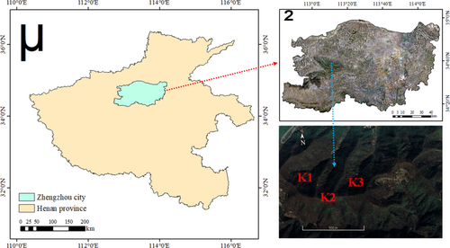
The natural environment conditions are good and the climate is warm and humid. The maximum rainfall during the process can reach more than 100 mm, and a large amount of rainwater permeates into the ground along the cracks, speeding up the weathering speed of the rocks. The slope gradient and height are 36°˜70° and 150˜250 m respectively. The rock and soil of the slope are mainly silty clay, limestone, and granite porphyry. The change of stratum attitude is greatly affected by the structure. The rock mass structure is complete, and there is no fault fracture zone and few discontinuous structural planes.
3 Methods
3.1 Evaluation Index System
Slope stability is often influenced by the interaction and coupling of multiple evaluation indexes, some of which are interrelated, leading to redundant information representation that can affect the final evaluation outcomes [21, 22]. Therefore, this paper reviews the current studies on slope stability evaluation, and qualitatively and quantitatively screens the summarized indexes [23, 24].
3.1.1 Qualitative Screening
- Scientificity: the primary condition of index selection is scientific, which needs to refer to a large number of references to choose;
- Rationality: the selection of indexes can objectively evaluate the slope;
- Representativeness: the selection of indexes should be as comprehensive as possible and have certain representativeness, covering all aspects of characteristics related to slope stability;
- Feasibility: the source of index data should be reasonable, the definition should be accurate, and the acquisition of index value has a certain convenience.
3.1.2 Quantitative Screening
3.2 Determination of the Weight of Evaluation Indexes
3.2.1 Improve Analytic Hierarchy Process
Analytic hierarchy process (AHP) is often applied to obtain the subjective weight of indexes in risk assessment [26]. The traditional AHP calculates the index weight by constructing the judgment matrix, which requires a consistency check. To address this limitation, this paper uses the weight coefficient to improve it, and optimizes the matrix with the optimal transfer matrix, which does not need a consistency check, so as to avoid the situation that the consistency is not satisfied [27, 28].
3.2.1.1 Judgment Matrix
| Take a value | Meaning |
|---|---|
| 1 | Si is as important as Sj |
| 3 | Si and Sj are slightly more important |
| 5 | Si and Sj are obviously important |
| 7 | Si and Sj are strongly important |
| 9 | Si and Sj are extremely important |
3.2.1.2 Antisymmetric Matrix
3.2.1.3 Quasi-Optimal Transitive Matrix
3.2.1.4 Weight Coefficient
3.2.2 Anti-Entropy Weight
Entropy weight can obtain weights according to the situation of index data, which effectively reduces the impact of subjective factors in the process of weight determination [29]. However, when determining weights, the entropy weight method will amplify the weights of individual indexes, and the weights obtained are prone to significant fluctuations due to variations in individual indexes [30].
Anti-entropy weight (AEW) is an improvement based on entropy weight theory, which effectively avoids extreme weight outcomes during the weight determination process using the entropy weight method, resulting in more accurate weight calculations [31, 32]. The weight determination steps are as follows:
3.2.2.1 Evaluation Index MATRIX
3.2.2.2 Anti-Entropy of Each Evaluation Index
3.2.2.3 Objective Weight
3.2.3 Game Theory
The improved AHP mainly evaluates the relative importance according to experience, which may lead to the influence of the objective value of the evaluation index on the evaluation results being overlooked [33]. Anti-entropy weight completely depends on the original data of the evaluation index, so the final calculated result may not be consistent with reality [34]. To make full use of their advantages and avoid their respective defects, this paper uses game theory to integrate them.
3.3 Determination of Stability Level Based on Improved Cloud Matter-Element Model
3.3.1 Finite Interval Cloud Model
Cloud model is a mathematical theory developed on the basis of fuzzy mathematics and statistics to describe the relationship of uncertainty [38]. It combines uncertainty, fuzziness, and randomness to form a mapping relationship between qualitative and quantitative description [39]. It is commonly employed in evaluation and prediction in different engineering fields. The stability of slope has the feature of uncertainty and fuzziness. The traditional cloud model requires that the evaluation index conforms to the characteristics of a normal distribution, which may not always correspond to actual conditions [40].
3.3.2 Theory of Matter Element
In order to explore the intrinsic law of change of things as well as mutual influence, Cai Wen put forward the concept of matter-element theory in the 1980s. The core of this theory is the use of a correlation function to describe the degree to which a system belongs to a certain nature or category [45]. Matter-element theory regards matter-element as its fundamental constituent.
3.3.3 Improved Cloud Matter-Element Model
The conventional cloud matter-element model is formed by fusing the matter-element model and cloud model. However, matter-element theory often employs fixed values or intervals to quantitatively describe various features of things, which can sometimes neglect the inherent fuzzy and random uncertainties in each feature's description. The finite interval cloud model not only encompasses the merits of the traditional cloud model, enabling effective handling of fuzziness and randomness, but also accounts for the inherent characteristics of limited interval distributions observed in the actual distribution of evaluation indexes.
3.4 The Implementation Process of the Slope Stability Evaluation Method
The proposed slope stability evaluation method is implemented through the following steps, and the research framework is shown in Figure 2.
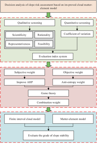
Step 1: Construction of the evaluation index system.
The evaluation indexes are first qualitatively screened based on the principles of scientific validity, rationality, representativeness, and feasibility. Subsequently, a quantitative screening is performed using the coefficient of variation to eliminate indexes with low information contribution, ensuring a concise and effective evaluation index system.
Step 2: Calculation of combined weights for evaluation indexes.
Subjective weights are derived using an improved analytic hierarchy process, while objective weights are obtained using the anti-entropy weight method. These two types of weights are then integrated through game theory, applying the principle of deviation minimization to determine the final comprehensive weight vector.
Step 3: Construction of the finite interval cloud model.
For each evaluation index under different stability grades, the (Ex En He) is calculated to serve as the three numerical characteristics of the cloud model. A cloud generator is then used to simulate a large number of cloud droplets, reflecting the uncertainty and fuzziness of each index across different grade intervals.
Step 4: Integration of cloud model and matter-element model.
The cloud numerical features (Ex En He) are embedded into the matter-element model to construct an improved cloud matter-element structure. The cloud correlation degree between each index and each stability grade is then calculated, reflecting the degree of association of the indexes with each grade.
Step 5: Comprehensive evaluation and multiple simulations.
Based on the comprehensive weight vector obtained in Step 2, the weighted sum of cloud correlation degrees is calculated to obtain a comprehensive slope stability score. To reduce the impact of randomness, multiple simulations are conducted (N = 1000), and the expectation of the evaluation results is taken as the final assessment value.
Step 6: Determination of stability grade and confidence factor.
The final slope stability grade is determined by comparing the comprehensive evaluation value against pre-defined grading intervals. Additionally, a confidence factor (θ) is calculated to evaluate the dispersion and reliability of the simulation results. A result is considered statistically reliable when θ < 0.01.
4 Results and Discussion
4.1 Evaluation Index System
In this paper, literatures on slope stability are combed out [50-54], and 12 evaluation indexes are qualitatively selected based on the principles of scientificity, rationality, representativeness, and feasibility, as shown in Table 2.
| Serial number | Index name |
|---|---|
| X1/MPa | Uniaxial compressive strength |
| X2 | Elasticity modulus |
| X3 | Poisson's ratio |
| X4/% | RQD |
| X5/MPa | Cohesion |
| X6/° | Internal friction angle |
| X7/mm | Maximum process rainfall |
| X8/L•min−1•10−1 m−1 | Underground seepage rate |
| X9/m | Slope height |
| X10/° | Slope |
| X11/° | Seismic intensity |
| X12/cm•s−1 | Blasting vibration velocity |
A large number of indexes will not only complicate the evaluation process, but also affect the distribution of index weights. Therefore, the coefficient of variation of each evaluation index is obtained according to Equations (1) and (2), and the evaluation index is screened, as shown in Figure 3.
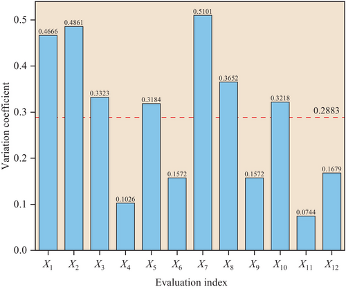
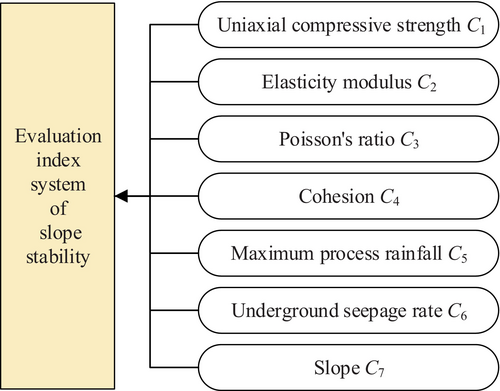
If the number of selected indexes is too large, there will be information redundancy among indexes and a large amount of calculation work. If the number is too small, the characteristics of slope stability cannot be fully expressed. Therefore, the evaluation indexes whose coefficient of variation is less than the average (2.8883) are eliminated in this paper, and 7 evaluation indexes were finally selected to construct the evaluation index system of slope stability, as shown in Figure 4.
4.2 Determination of the Weight
| Index weight | |||||||
|---|---|---|---|---|---|---|---|
| Weight determination | C1 | C2 | C3 | C4 | C5 | C6 | C7 |
| W1 | 0.1706 | 0.2900 | 0.0602 | 0.0469 | 0.2247 | 0.1293 | 0.0783 |
| W2 | 0.1493 | 0.1725 | 0.1308 | 0.1229 | 0.1675 | 0.1354 | 0.1216 |
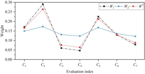
| W* | 0.1658 | 0.2638 | 0.0759 | 0.0639 | 0.2120 | 0.1306 | 0.0880 |
Then, on account of the calculation flow of anti-entropy weight theory, the objective weight W2 can be obtained by using Equations (9-11), as shown in Table 3.
Finally, the game theory is used to optimize W1 and W2, and the combination coefficients α1 = 0.7771 and α2 = 0.2229 are obtained; thus, the comprehensive weight W* values are obtained, as shown in Table 3.
When the weight method of the index is different, the weight result is also different, and the comparative analysis of weight value is shown in Figure 5. From the Figure 5, the comprehensive weight W* determined based on game theory is between subjective weight and objective weight, and the overall trend is consistent, indicating that the comprehensive evaluation takes into account both subjective factors from experts and the inherent characteristics of the index.
4.3 Determination of Stability Grade
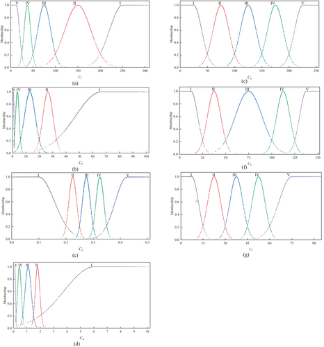
Before evaluating, the evaluation index needs to be classified. The slope stability is divided into five grades: extremely stable (I), stable (II), basic stable (III), unstable (IV) and extremely unstable (V) [55]. The classification criteria corresponding to each evaluation index are shown in Table 4. Based on the finite interval cloud model theory, the digital characteristics of the cloud model for each evaluation index are calculated using Equations (15-18). Then, a normal cloud generator program is developed in MATLAB, with the cloud model's digital characteristics and 4000 cloud droplets as inputs. This process produces a cloud map formed by the aggregation of cloud droplets in the numerical domain, thereby generating cloud model diagrams that represent the degree to which each index belongs to different stability levels, as shown in Figure 6.
| Evaluation index | Index name | ||||
|---|---|---|---|---|---|
| I | II | III | IV | V | |
| C1 | 200 ˜ 300 | 100 ˜ 200 | 50 ˜ 100 | 25 ˜ 50 | 0 ˜ 25 |
| C2 | 33 ˜ 100 | 20 ˜ 33 | 6 ˜ 20 | 1.3 ˜ 6 | 0 ˜ 1.3 |
| C3 | 0 ˜ 0.2 | 0.2 ˜ 0.25 | 0.25 ˜ 0.30 | 0.3 ˜ 0.35 | 0.35 ˜ 0.5 |
| C4 | 2.1 ˜ 10 | 1.5 ˜ 2.1 | 0.7 ˜ 1.5 | 0.2 ˜ 0.7 | 0 ˜ 0.2 |
| C5 | 0 ˜ 50 | 50 ˜ 100 | 100 ˜ 150 | 150 ˜ 200 | 200 ˜ 250 |
| C6 | 0 ˜ 25 | 25 ˜ 50 | 50 ˜ 100 | 100 ˜ 125 | 125 ˜ 150 |
| C7 | 0 ˜ 15 | 15 ˜ 30 | 30 ˜ 45 | 45 ˜ 60 | 60 ˜ 90 |
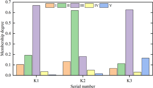
According to the grading standards in Table 4, the certainty degree of each evaluation index belonging to different stability levels is calculated by Equations (15-19). Then, according to the comprehensive weight obtained by game theory and the improved cloud matter-element model, the comprehensive evaluation value of each slope is calculated according to Equations (22-24), as shown in Figure 7. Due to the strong randomness in the process of solving cloud correlation degree, the expected value of numerous data needs to be solved several times to reduce the impact of random errors. In this paper, the number of solving N = 1000 is set, so as to finally obtain the comprehensive evaluation value and confidence factor of each slope, as shown in Table 5.
| Serial number | Confidence factor | Comprehensive evaluation value | Stability grade | Ture result |
|---|---|---|---|---|
| K1 | 0.0006 | 2.6364 | III | III |
| K2 | 0.0015 | 2.1986 | II | II |
| K3 | 0.0007 | 3.1140 | III | III |
According to Table 5, the confidence factors of the three slopes are all less than 0.01, which indicates the correctness of the evaluation results. Besides, the stability levels of slope K1 and K3 are basically stable (III), and the stability level of K2 is stable (II), meeting the requirements of engineering construction stability and not prone to geological disasters. The evaluation results align perfectly with the actual investigation findings, confirming the effectiveness and feasibility of the slope stability evaluation model, and has certain practical value in engineering.
5 Discussion
Based on game theory and a finite interval cloud matter-element model, this paper develops an integrated and novel approach for slope stability evaluation. First, to construct a rational and concise index system, evaluation indexes were screened both qualitatively and quantitatively using a combination of expert-driven principles and the coefficient of variation, effectively eliminating redundancy while retaining key influencing factors. Second, a significant methodological advancement lies in the comprehensive weighting mechanism: unlike traditional studies that apply either subjective or objective weighting alone, we combine improved analytic hierarchy process and anti-entropy weighting through game theory. This ensures optimal weight fusion by minimizing deviations between methods, achieving a better balance between expert judgment and objective data distribution. In terms of evaluation model, we innovate by integrating the finite interval cloud model into matter-element theory, thereby enabling the conversion between qualitative uncertainty and quantitative data. By employing the cloud model's numerical characteristics—expectation (Ex), entropy (En), and hyper-entropy (He)—as substitutes for static feature values in the matter-element model, the approach captures both fuzziness and randomness in slope, which traditional methods fail to address adequately. Furthermore, to enhance the robustness of evaluation results, we replace the conventional maximum membership principle with an expectation-based multi-simulation strategy. By repeatedly solving the model (N = 1000), the average outcome is taken as the final stability grade, which effectively reduces the influence of randomness, resolves boundary ambiguity in classification, and allows for a more stable and interpretable visualization of slope stability levels. Collectively, this approach not only improves the scientific rigor of multi-criteria decision-making under uncertainty but also offers significant theoretical innovation and practical applicability in geotechnical engineering risk assessment. The evaluation model established in this paper is generally applicable to the stability evaluation of various types of slopes. Although the core algorithm is universal, the index system can be flexibly adjusted according to the specific characteristics of different slope types. Meanwhile, cloud model parameters such as the entropy interval boundary can be refined to better capture different geotechnical mechanical properties.
According to the results in Table 5, the stability level of the slope can be intuitively seen, and it can make the evaluation level of the object to be evaluated more intuitive, highlighting the advantages of this evaluation model. According to the evaluation results, the stability levels of slope K1 and K3 are basically stable, and the stability level of K2 is stable. In order to prevent the transformation from basically stable to unstable, reinforcement measures should be taken in time to optimize the blasting mode, reduce the disturbance and damage effect of blasting on the slope, and at the same time, the design of the anti-drainage system should be done well to avoid the phenomenon of slope instability.
6 Conclusions
- The indexes are screened based on the principle of index screening and coefficient of variation, and the indexes that have no significant influence on the evaluation results are eliminated, and an evaluation index system of slope stability is constructed.
- The evaluation indexes are weighted subjectively and objectively by using the improved AHP and the anti-entropy weight theory, and the weights are fused based on game theory. As a result, the comprehensive weights of the seven indexes are 0.1658, 0.2638, 0.0759, 0.0639, 0.2120, 0.1306, and 0.0880, respectively. Combination weighting avoids the defect of single index weighting and improves the accuracy and rationality of index weight determination.
- The finite interval cloud model and matter-element model are combined to evaluate the stability of slope, which effectively solves the fuzziness and randomness. The results show that the stability levels of slope K1 and K3 are basically stable, the stability level of K2 is stable, and the evaluation results are consistent with the actual project, which verifies the correctness of the evaluation model.
Author Contributions
Wan-Rui Hu: formal analysis, conceptualization, software, writing – original draft, investigation. Heng Liu: investigation, conceptualization, methodology, writing – review and editing, software. Xing-Tao Zhou: formal analysis, methodology, writing – review and editing, investigation, conceptualization, software. Bo Wei: formal analysis, methodology, software, conceptualization. Ceng Shang: investigation, writing – review and editing, validation, methodology, formal analysis. Peng Guan: conceptualization, writing – review and editing, formal analysis, software.
Acknowledgments
This work was supported by the China Postdoctoral Science Foundation (Grant No. 2024M752746 and No. 2024T170760), and the Natural Science Foundation of Hubei Province, China (Grant No. 2025AFB888).
Conflicts of Interest
The authors declare no conflicts of interest.
Open Research
Data Availability Statement
Data sharing not applicable to this article as no datasets were generated or analysed during the current study.


