Transformer fault diagnosis is crucial for the safe operation of power systems, enabling quick and accurate fault type identification. However, traditional methods struggle with extracting multi-scale temporal features and high-order feature representations, limiting their ability to handle complex dynamic data patterns. To address this, this paper proposes a multi-scale temporal adaptive fusion network (MSTAFN). The MSTAFN model first generates a time position vector through a temporal information encoding (TIE) module, capturing multi-scale temporal features. The adaptive high-order hybrid network (AHOHN) module then fuses multi-scale temporal data with transformer features using a hybrid attention mechanism, extracting temporal variation patterns. To enhance high-order feature representation, the high-order feature extraction (HOFE) module introduces nonlinear activation and higher-order operations to capture complex relationships between features. The adaptive feature reconstruction (AFR) module dynamically adjusts the feature fusion ratio, optimizing information integration. Finally, the multi-scale temporal fusion (MSTF) module balances the fusion of multi-scale temporal features and global dependencies, adapting to different tasks and data distributions. Extensive experiments on publicly available datasets demonstrate that the MSTAFN model outperforms comparison models across multiple evaluation metrics, proving its effectiveness and superiority in transformer fault diagnosis.

1 Introduction

Power transformers are core components of modern power systems, and their operational status directly affects the safety and stability of the entire system. However, due to the complex operating environment and diverse fault types of transformers, accurate fault diagnosis is crucial for ensuring their stable operation [1, 2]. Traditional fault diagnosis methods for power transformers include frequency response analysis (FRA) [3], short circuit reactance (SCR) [4], low-voltage impulse (LVI) [5], and ultrawideband (UWB) methods [6]. While each of these methods has its advantages, they also have certain limitations. For instance, dissolved gas analysis (DGA) and vibration analysis are two common diagnostic techniques. DGA identifies fault types by analyzing the composition and ratio of dissolved gases, making it suitable for oil-immersed transformers, but it cannot be applied to dry-type transformers. On the other hand, vibration analysis is mainly used to detect mechanical issues such as winding looseness or core problems, but it may not effectively diagnose other types of faults.

With the development of machine learning and sensor technologies, intelligent algorithms such as support vector machines (SVM) [7], Bayesian networks [8], and extreme learning machines (ELMs) [9] have been applied to transformer fault diagnosis. However, these methods are mainly based on shallow learning algorithms. Although they can improve diagnostic accuracy to some extent, their data analysis capabilities are relatively weak, and their performance in real-world industrial environments is limited. In contrast, deep learning methods have become the mainstream approach for transformer fault diagnosis due to their powerful learning and feature extraction capabilities. Common deep learning networks, such as deep belief networks (DBNs) [10], long short-term memory (LSTM) networks [11], and convolutional neural networks (CNN) [12], have been widely applied in the field of fault diagnosis.

However, traditional CNNs suffer from the degradation problem when increasing network depth, which negatively impacts the model's diagnostic performance. To address this issue, He et al. proposed residual networks (ResNet) [13], which significantly alleviate the degradation problem of deep networks by introducing residual modules with shortcut connections. The ResNet structure has been proven to perform exceptionally well in fault diagnosis and has become a widely used tool in this field [14-18]. In addition to CNNs and ResNets, graph convolutional networks (GCNs) [19-21] have also been applied in transformer fault diagnosis. By constructing a graph structure and extracting high-order features, GCNs can capture the complex nonlinear relationships between dissolved gases and fault types, offering higher diagnostic accuracy and generalization ability when dealing with small samples and complex data.

In recent years, attention mechanisms have been widely used in transformer fault diagnosis [22-24], as they help focus on key features while suppressing irrelevant information. Zhou et al. [22] proposed a fusion residual attention diagnostic (FRAD) model, which generates and fuses vibration signal images through the design of a Gramian-guided filtering module (GGFM) and improves the deep ResNet by introducing an up-dimensioning convolutional block attention module (UCBAM), thereby enhancing the accuracy of power transformer fault diagnosis. Ding et al. [23] proposed a time–frequency transformer (TFT) model, designing a new tokenizer and encoder module to extract effective features from the time-frequency representation of vibration signals, and constructed an end-to-end fault diagnosis framework based on the TFT. However, these attention-based methods have limitations in multi-scale temporal feature extraction, primarily because they lack an effective time information encoding mechanism. They often rely on fixed attention mechanisms that cannot flexibly adapt to changes across different time scales, making it difficult to consider subtle differences between time scales when processing complex dynamic data. Additionally, these methods struggle to effectively integrate complex interactions between high-order features, which are crucial in transformer fault diagnosis as they reveal deep nonlinear relationships within fault patterns. To address these limitations in traditional methods, this paper proposes the multi-scale temporal adaptive fusion network (MSTAFN).

The MSTAFN network first generates a time position vector through a temporal information encoding module, which effectively captures temporal variation features across different time scales. In the designed adaptive high-order hybrid network (AHOHN) module, a hybrid attention mechanism is employed to seamlessly integrate multi-scale temporal information with transformer data features, overcoming the limitations of traditional methods in handling complex dynamic data patterns. The module then introduces a high-order feature enhancement (HOFE) mechanism that utilizes nonlinear activation and higher-order operations to improve the expression of nonlinear relationships between features. This enhancement process allows the model to capture the complex interactions between high-order features better, compensating for the shortcomings of traditional methods in high-order feature extraction. Furthermore, the adaptive feature reconstruction (AFR) module dynamically adjusts the fusion ratio of different features based on varying data distributions and task requirements, optimizing the feature integration process. Finally, the multi-scale temporal fusion (MSTF) module dynamically balances the fusion of multi-scale temporal features with global dependencies, further improving the integration of information and ultimately increasing fault diagnosis accuracy. Experimental results demonstrate that the MSTAFN model outperforms comparative models across various evaluation metrics on publicly available transformer fault datasets, validating its effectiveness and superiority in transformer fault diagnosis. The contributions of this paper are as follows:

The time information encoding module introduces learnable parameters and a dynamic modulation mechanism, allowing the encoding process to adjust frequency and phase based on specific fault data. This enables better capture of multi-scale dynamic relationships and effectively represents nonuniform periodicity and complex behaviors.
The AHOHN module is designed to integrate temporal and data features using a hybrid attention mechanism to capture multi-scale variations. The HOFE module deepens feature interactions through nonlinear activation and higher-order operations. The AFR module is applied to dynamically adjust feature fusion, optimizing the integration process for different tasks and data.
The MSTF module uses an adaptive fusion factor to adjust the contribution ratio between BiGRU and multi-scale memory residual network (MSMRN) features, ensuring optimal integration of temporal modeling and multi-scale feature extraction. Experimental results show that the MSTAFN method outperforms comparison models across various metrics, demonstrating its effectiveness and superiority.

2 Related Work

2.1 Diagnosis Method Based on Physical Principles

Pramanik et al. [3] proposed an innovative FRA method for detecting transformer winding faults, using two sinusoidal excitations with equal amplitude but opposite polarity. This method compares the impedance response differences between the two ends of the transformer, without needing a healthy reference. Palani et al. [4] introduced a fault detection method that combines real-time voltage, current, and power comparisons with high-resolution sampling, allowing accurate detection of winding faults during short-circuit tests without reference data. Christian et al. [5] expanded detection methods using three transfer function-based approaches, offering new ways to detect mechanical displacement in transformers. Similarly, Mortazavian et al. [6] proposed a fault detection method based on SAR imaging and Kirchhoff migration algorithms, effectively detecting mechanical deformations in high-voltage transformer windings.

While these methods can identify faults without healthy data, their applicability is limited by specific experimental setups and data conditions. Additionally, factors like winding design and aging may affect detection accuracy across different transformers or operating conditions.

2.2 Diagnosis Methods Based on Machine Learning

Zhang et al. [14] further introduced a wide ResNet method with incremental learning capability, allowing the model to continue learning and optimizing as new fault data becomes available, enhancing its adaptability. Xing et al. [15] developed a multi-modal deep residual filtering network (DRFN) for online fault diagnosis of T-type three-level inverters, which improves fault recognition accuracy by integrating multi-modal information. Xiong et al. [16] designed an adaptive denoising residual network (AD-ResNet), which improves fault diagnosis accuracy for rudder actuators by removing noise interference. Gituku et al. [17] apply refined composite multi-scale fuzzy entropy (RCMFE) for feature extraction and employ a self-organizing fuzzy (SOF) classifier for cross-domain fault diagnosis of bearings.

While these methods have made significant contributions to fault diagnosis in various devices, they often fail to autonomously focus on key information directly related to fault recognition. Instead, they are more likely to be influenced by irrelevant or noisy data, which can reduce diagnostic accuracy and generalization capability.

2.3 Hybrid Diagnostic Model Based on Deep Learning

In recent years, CNNs have driven the development of fault diagnosis methods using image processing. Liu et al. [18] proposed a motor fault diagnosis method based on multi-scale kernel residual CNN, enhancing fault sensitivity. Li et al. [19] converted vibration signals into 2D images and applied semi-supervised learning for fault diagnosis in rotating machinery. Wang et al. [25] used a symmetric point pattern (SDP) to generate images for bearing fault classification, demonstrating the effectiveness of image-based approaches. Hong et al. [26] applied CNN to vibration images for transformer fault diagnosis.

Researchers have further improved diagnosis accuracy by integrating attention mechanisms. Zhou et al. [22] proposed a FRAD model, using a Gramian-guided filtering module to fuse vibration signal images with a deep ResNet for transformer fault detection. Ding et al. [23] introduced a TFT model to extract features from vibration signals' time-frequency representation, creating an end-to-end diagnosis framework. Gangtao et al. [24] combined 1D-CNN and channel attention mechanisms for transformer fault detection and used generative adversarial networks (GANs) to address data limitations, improving performance and generalization.

These methods have significantly advanced fault diagnosis, especially by combining image processing with deep learning and attention mechanisms, boosting accuracy and adaptability to complex fault patterns.

3 Methods

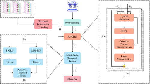
The MSTAFN model framework is shown in Figure 1. First, the temporal position vector is obtained through the temporal information encoding module. The transformer data features and time position vector are then input into the AHOHN module, which uses hybrid attention to integrate temporal and data features, capturing correlations between time steps and features. HOFE module captures complex nonlinear relationships to improve feature representation. Next, the adaptive feature fusion module dynamically adjusts the fusion ratio based on feature importance, optimizing information integration. Residual connections retain original features and enhance information flow. The data then passes through the MSTF module, where a BiGRU captures bidirectional temporal dependencies, and the MSMRN extracts multi-scale global features. Then the adaptive fusion module combines the outputs of the BiGRU and MSMRN, optimizing the contribution of each feature for efficient understanding and accurate predictions. Finally, the results are output through the classifier.

Details are in the caption following the image — **FIGURE 1**
Open in figure viewer PowerPoint

The framework of the MSTAFN model.

3.1 Temporal Information Encoding

Traditional time position encoding methods use fixed frequency distributions, making it difficult to adapt to specific tasks or data characteristics, especially in transformer fault diagnosis. This limits their ability to capture complex nonlinear relationships and multi-scale variations in nonstationary time series. To overcome this, we propose an adaptive trigonometric position encoding method. By introducing learnable parameters and a dynamic modulation mechanism, the model can adjust frequency and phase to better capture complex temporal features. The trigonometric functions provide nonlinearity, and the learnable parameters help the model adapt to multi-scale dynamic relationships, improving fault diagnosis accuracy and robustness. The calculation formula is shown in Equation (1)

P{E}_{\left( pos,2i\right)}=\sin \left(\frac{\alpha_i\cdotp pos+{\beta}_i}{f_i(d)}\right),P{E}_{\left( pos,2i+1\right)}=\cos \left(\frac{\alpha_i\cdotp pos+{\beta}_i}{f_i(d)}\right)

(1)

where

pos

represents the position index in the time series, indicating the time location.

{\alpha}_i

and

{\beta}_i

are learnable parameters, where

{\alpha}_i

adjusts the frequency to capture different time cycle features, and

{\beta}_i

adjusts the phase shift, improving the model's ability to express nonlinear characteristics. The modulation function

{f}_i(d)

, related to the input feature dimension

d

, normalizes the frequency and phase across multiple scales, enabling dynamic adaptation to the input data and capturing multi-scale temporal patterns and complex dynamics. The calculation of

{f}_i(d)

is shown in Equation (2)

{f}_i(d)=\frac{\sqrt{d+1}}{1+\beta \cdotp \log \left(1+d\right)}

(2)

The learnable parameter $\beta$ controls the scaling and adjustment effect on the input $d$ . This modulation function smoothly adapts to the nonlinear growth characteristics of high-dimensional data, while enabling multi-scale normalization. It effectively prevents the excessive growth of high-dimensional features, ensuring numerical stability and enhancing the robustness of the model.

3.2 Adaptive High-Order Hybrid Network

3.2.1 Hybrid Attention

The hybrid attention mechanism integrates both time position information and data features, enabling the model to capture global long-term dependencies as well as local short-term variations. This improves the model's ability to represent features comprehensively, preventing information bias or the loss of important dimensions. The computation process is illustrated in Equation (3)

{H}_a={A}_m\left({Q}_d,{K}_d,{V}_d,{Q}_t,{K}_t\right)=\mathrm{Softmax}\left(\frac{Q_d{K_d}^T+{Q}_t{K_t}^T}{\sqrt{d_k}}\right){V}_d

(3)

The values ${Q}_d$ , ${K}_d$ , and ${V}_d$ are derived from the data features ${H}_d$ , while ${Q}_t$ and ${K}_t$ are computed from the time position vectors ${H}_t$ . ${d}_k$ is the feature dimension of ${Q}_d$ . After their summation, the hybrid attention mechanism effectively integrates both the time position and data feature dependencies, capturing dynamic relationships while incorporating both background dynamics and key patterns. By combining the data feature vectors, a unified feature representation is generated, providing high-quality input for subsequent tasks and enhancing the model's expressive power.

3.2.2 High-Order Feature Enhancement

Traditional methods often fail to capture higher-order nonlinear relationships and multimodal interactions between features, limiting the model's ability to handle dynamic changes and diverse feature combinations. To overcome this, we introduce the HOFE module. Building on the output of the hybrid attention mechanism, the HOFE module uses nonlinear activation and element-wise higher order operations to further explore the relationships and interactions between input features. The HOFE module enhances feature representation by emphasizing higher order interactions. This not only strengthens the nonlinear expression of features but also compensates for interactions that may be missed by the attention mechanism, improving the model's ability to adapt and perform robustly in complex data scenarios. The computation of HOFE is shown in Equation (4):

{H}_h=\sigma \left({W}_a\cdotp {H}_a+{b}_a\right)+\lambda \cdotp \left({H}_a\odot {H}_a\right)

(4)

Here, ${W}_a$ represents the learnable weight vector, ${b}_a$ denotes the bias vector, and ReLU is applied as the activation function $\sigma$ . $\lambda$ is a tunable hyperparameter that controls the contribution of the higher order feature interaction to the final feature representation.

3.2.3 Adaptive Feature Reconstruction

The HOFE module improves feature representation by capturing nonlinear interactions. However, not all tasks or fault scenarios require high-order features equally. Using enhanced features directly may cause overfitting or neglect important first-order information. To address this, the AFR module is introduced. It dynamically adjusts the fusion of high-order and original features based on their importance. In complex fault scenarios with strong feature interactions, it prioritizes high-order features, while in simpler scenarios, it retains key first-order features. This dynamic adjustment improves model robustness and flexibility, enhancing diagnosis accuracy. The AFR module's computation process is outlined in Equations (5) and (6)

\alpha =\mathrm{Sigmoid}\left({W}_{\alpha}^{\top }{H}_a\right),\beta =\mathrm{Sigmoid}\left({W}_{\beta}^{\top }{H}_a\right)

(5)

{H}_{\mathrm{r}}=\alpha \cdotp {H}_{\mathrm{h}}+\beta \cdotp {H}_a

(6)

The weights $\alpha$ and $\beta$ are dynamically determined by the fusion of the original features, allowing for flexible adjustment based on task requirements. ${W}_{\alpha}^{\top }$ and ${W}_{\beta}^{\top }$ represent the learnable weight vector. $\mathrm{Sigmoid}$ is used as an activation function. Specifically, when fault patterns exhibit clear feature interactions, such as the complex coupling between dissolved gas concentration, temperature, and current, the weight $\alpha$ increases, emphasizing the role of high-order features. This helps the model more accurately capture these intricate interactions. In contrast, in simpler fault scenarios, such as those characterized solely by an increase in gas concentration, the weight $\beta$ decreases, highlighting the importance of original features and preserving essential first-order information to avoid unnecessary complexity.

3.3 Multi-Scale Temporal Feature Fusion

3.3.1 BIGRU Model

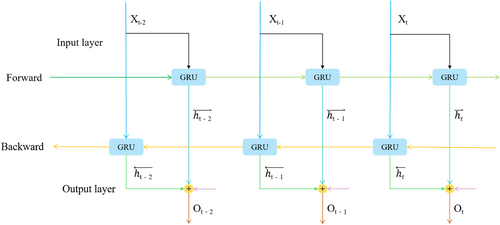
The network framework of the BiGRU is shown in Figure 2. In transformer fault diagnosis, after the AHOHN has processed the data, complex feature extraction and nonlinear relationships have been modeled. However, these features still lack a comprehensive capture of temporal information. To address this issue, the BiGRU model is employed to process both forward and backward temporal information, allowing the model to fully exploit bidirectional dependencies within the feature sequence. This compensates for the important contextual information that might be missed in a unidirectional network. Specifically, the BiGRU can capture the dynamic changes and long-term dependencies of fault signals, enhancing the model's ability to model temporal features. In scenarios where the transformer undergoes gradual aging or when fault characteristics exhibit periodic fluctuations, the BiGRU can more accurately identify fault patterns.

3.3.2 MSMRN Model

The MSMRN models data from different time windows through a multi-scale mechanism, enabling the capture of relationships between short-term local features and long-term global trends. At the same time, the ResNet effectively mitigates the vanishing gradient problem through skip connections, ensuring the training stability of deep networks and enhancing the model's ability to express nonlinear features. The structure of the MSMRN is shown in Figure 3.

Specifically, the MSMRN preserves key fault features at different time scales, enhancing its ability to recognize transformer fault patterns. It captures multilevel variations in fault signals during transformer operation, such as the coupling of short-term fluctuations with long-term trends. This improves the accuracy and robustness of fault diagnosis, providing more comprehensive support for transformer condition assessment and fault prediction.

3.3.3 Adaptive Temporal Fusion

The BiGRU and MSMRN modules each have unique advantages in transformer fault diagnosis. BiGRU excels at extracting temporal features of transformer fault signals, capturing time dependencies and dynamic variations in the data. On the other hand, the MSMRN model focuses on multi-scale feature modeling, enabling it to capture both short-term local variations and long-term global trends in the signal. While both modules offer distinct strengths, using them individually may lead to the neglect of certain important features, limiting the comprehensive representation of fault characteristics.

To address this issue, we have designed an adaptive temporal fusion module to dynamically integrate the output features of BiGRU and MSMRN. This module calculates an adaptive fusion factor that adjusts the contribution ratio of the two features based on the characteristics of the input data. This approach not only preserves the temporal modeling capability of BiGRU and the multi-scale feature advantage of the MSMRN model but also dynamically optimizes their fusion ratio based on actual needs. This ensures that the fused features comprehensively and accurately represent the complexity of transformer fault signals. The specific calculation process is shown in Equations (7-9)

{H}_c= concat\left({H}_G;{H}_M\right)

(7)

\alpha =\sigma \left({W}_{\alpha }{H}_c+{b}_{\alpha}\right)

(8)

{H}_f=\alpha \cdotp {H}_c+\left(1-\alpha \right)\cdotp {H}_G

(9)

where

{H}_G

and

{H}_M

represent the output results from the BiGRU and MSMRN modules, respectively.

concat

is the feature concatenation operation.

{W}_{\alpha }

is the learnable weight coefficient.

{b}_{\alpha }

is the bias term. In transformer fault diagnosis tasks, this fusion approach effectively overcomes the limitations of modeling features in isolation. By integrating temporal features with multi-scale features, the module significantly enhances the understanding of complex fault patterns. This not only improves the accuracy of fault diagnosis but also strengthens the robustness of the diagnostic model, providing reliable technical support for precise fault identification and early warning in complex fault scenarios.

3.4 Classifier

We use depthwise separable convolution as the classifier, as this module efficiently extracts local features while reducing computational complexity. Transformer fault signals typically exhibit significant local characteristics, such as abnormal fluctuations or abrupt changes, which are crucial for accurately identifying fault patterns. Depthwise separable convolution decomposes the traditional convolution operation into depthwise convolution and pointwise convolution, significantly reducing both computation and parameter count. This design not only enhances the model's efficiency in handling large-scale data but also preserves its strong feature representation capability. The computation process is shown in Equation (10)

{D}_f= DWConv\left({H}_f\right)

(10)

4 Experiments and Result Analysis

4.1 Dataset

This study conducts experimental analysis based on a 220 kV voltage dataset from the State Grid Corporation of China and previous literature [27, 28]. The dataset includes multiple features, such as the concentrations of dissolved gases (H₂, CH₄, C₂H₂, C₂H₄, C₂H₆). In the data preprocessing stage, we performed data cleaning and retained 718 valid samples. These samples represent seven distinct fault states: Normal, Low-Temperature Overheating, Medium-Temperature Overheating, High-Temperature Overheating, Partial Discharge, Low Energy Discharge, Low Energy Discharge With Overheating, High Energy Discharge, and High Energy Discharge With Overheating.

To train and evaluate the model performance, we first sorted the dataset chronologically and then split it into a training set and a testing set in an 8:2 ratio, with 80% of the samples used for training and 20% for testing. The sample distribution across different fault states is shown in Table 1. By splitting the dataset in this time-sequenced manner, we ensured data independence, avoiding future data leakage, and enabling a comprehensive evaluation of the model's generalization ability and predictive performance across various fault states.

TABLE 1. Sample distribution of the dataset.

Status	All samples	Training samples	Testing samples
Normal	52	40	12
LT	99	80	19
MT	73	58	15
HT	168	134	34
PD	105	84	21
LD	42	34	8
HD	179	143	36

4.2 Experimental Setup

The MSTAFN model was implemented using the PyTorch framework and trained on an NVIDIA GeForce GTX 1080 Ti GPU. The model parameters were determined through multiple comparative experiments. During training, the batch size was set to 64, and the model was trained for a total of 100 epochs. The Adam optimizer was used with an initial learning rate of 0.001. The convolutional kernels of the MSMRN were set as [1 × 1, 3 × 1, 5 × 1], and the weight parameter $\lambda$ for high-order features was set to 0.45.

4.3 Loss Function

The cross-entropy loss function was chosen as the loss function for the MSTAFN model because it is well-suited for classification tasks, especially multi-class classification. This function measures the difference between the predicted probabilities and the true labels, guiding the model to learn accurate decision boundaries while maintaining stability during the optimization process. It helps improve both the model's performance and convergence speed. The computation of this loss function is shown in Equation (11)

\mathrm{Loss}=-\sum \limits_{i=1}^C\kern0.1em {y}_i\mathit{\log}\left({\hat{y}}_i\right)

(11)

where

C

is the number of categories,

{y}_i

is the one-hot encoding of the true labels, and

{\hat{y}}_i

is the predicted probability distribution from the model.

4.4 Evaluation Metrics

To comprehensively evaluate the performance of the proposed MSTAFN model, we use the following evaluation metrics: Accuracy (A), Precision (P), Recall (R), and F1 score. These metrics are used to measure the difference between the model's predicted values and the actual values. The formulas for each metric are provided in Equations (12-15)

A=\frac{TP+ TN}{TP+ FP+ TN+ FN}

(12)

P=\frac{TP}{TP+ FP}

(13)

R=\frac{TP}{TP+ FN}

(14)

F1=\frac{2\times P\times R}{P+R}

(15)

where

TP

is the true positive,

TN

is the true negative,

FP

is the false positive, and

FN

is the false negative.

4.5 Results and Analysis

4.5.1 Comparative Experiments

The performance metrics results of the proposed MSTAFN model and the comparison model on the transformer fault dataset are shown in Table 2. The experimental results show that the MSTAFN model achieved optimal performance across all evaluation metrics, including A, P, R, and F1, with values of 81.29%, 84.97%, 84.67%, and 84.82%, respectively. Compared to the best-performing GCN model, MSTAFN improved A, P, R, and F1 by 1.98%, 3.56%, 4.00%, and 3.78%, respectively. These significant improvements are attributed to the innovative design of MSTAFN and its comprehensive modeling of deep features. Traditional models often fail to effectively extract complex features or model relationships between samples, leading to poor performance on complex data. For example, XGBoost has an accuracy of only 64.14%, the lowest among all models, while KNN, though slightly better than other traditional methods, still shows a significant gap compared to deep learning models. This highlights the limitations of traditional methods in dynamic feature modeling and capturing complex patterns. CNNs, by using convolution operations, can extract local features but fail to effectively model global relationships between samples. Siamese networks improve performance by modeling the similarity between pairs of samples, but they still have limited capability in capturing global feature interactions. In contrast, GCNs model the global relationships between samples using adjacency vectors, significantly improving the understanding of the data structure, with an accuracy of 79.31%. However, GCN still struggles to capture the complex dynamic patterns in the data, showing limitations in dynamic temporal feature modeling.

TABLE 2. Comparison results of all the models.

Model	A (%)	P (%)	R (%)	F1 (%)
MLP [29]	67.21	70.17	69.67	69.92
XGBoost [30]	64.14	67.59	66.19	66.88
SVM [31]	68.79	71.54	69.46	70.48
KNN [32]	70.04	72.46	71.59	72.02
CNN [33]	75.63	78.52	77.27	77.89
Siamese Network [34]	77.13	79.53	78.34	78.93
GCN [20]	79.31	81.41	80.67	81.04
MSTAFN	81.29	84.97	84.67	84.82

MSTAFN effectively overcomes these challenges through its innovative design. First, the time information encoding module uses learnable parameters and dynamic modulation mechanisms to capture complex temporal features, addressing the limitations of other models in temporal dynamics modeling. Unlike traditional methods such as CNN and GCN, MSTAFN can more flexibly capture multi-scale temporal features, compensating for GCN's shortcomings in capturing dynamic patterns. Second, the AHOHN module captures complex nonlinear relationships through deep interaction between time positions and data features, significantly enhancing feature modeling capabilities. This makes MSTAFN superior to GCN and other methods in modeling higher order relationships. Furthermore, the multi-scale time fusion module, combining BiGRU and MSMRN, excels in capturing multi-scale temporal information and global dependencies, further improving the model's adaptability to complex dynamic data. Finally, the adaptive feature fusion module dynamically adjusts the fusion ratio of different features, ensuring the efficiency and robustness of the information integration process, which gives MSTAFN an advantage over other models in dynamic feature modeling. The synergistic effect of these modules enables MSTAFN to better model dynamic temporal features and high-order relationships in complex data.

4.5.2 Ablation Study

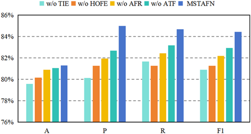
To further validate the role of different modules in the MSTAFN model, we removed or replaced one of the modules and compared the results with the complete MSTAFN model.

$w/o$ TIE: The temporal information encoding module was removed.
$w/o$ HOFE: The high-order feature enhancement module was removed.
$w/o$ AFR: The adaptive feature reconstruction was removed.
$w/o$ ATF: The adaptive temporal fusion was replaced with the traditional concatenation and linear operations.

Figure 4 shows the classification results of the proposed MSTAFN model and its submodules on transformer fault data. From Figure 4, the following conclusions can be drawn:

In transformer fault diagnosis, the TIE module incorporates time position information through learnable parameters and dynamic modulation mechanisms, effectively capturing complex temporal features such as frequency and phase. This compensates for the limitations of traditional models in dynamic time modeling. Removing this module significantly weakens the model's ability to capture key temporal features, especially when dealing with dynamic changes in frequency and phase, thus reducing diagnostic accuracy and reliability.
After integrating data features with temporal information, the HOFE module strengthens high-order interactions between features, enabling the capture of complex dynamic patterns and enhancing the model's ability to express nonlinear relationships. It significantly improves the model's adaptability and robustness in nonlinear fault scenarios, such as frequency drift and abrupt signal changes. Without the HOFE module, the model struggles to capture complex feature interactions, leading to reduced diagnostic accuracy for nonlinear fault patterns and instability in high-noise or complex scenarios, ultimately affecting overall fault diagnosis performance.
The AFR module uses a dynamic weighting mechanism to balance high-order and original features, improving the model's adaptability and diagnostic accuracy across diverse fault scenarios. Without it, the model fails to adjust the feature fusion ratio, resulting in poor representation of key features in complex and simple scenarios and reducing overall diagnostic performance.
The adaptive time fusion module dynamically adjusts the contribution of higher-order features and original features, effectively handling the complex dynamic patterns in transformer faults. Compared to traditional concatenation and linear transformation methods, it captures nonlinear relationships and deep interactions in time-series data more effectively. By optimizing the feature fusion strategy, this module significantly enhances the model's accuracy, especially when dealing with varying fault patterns.

4.5.3 The Impact of Different $\lambda$ Values on Classification Results

The experimental results for different high-order feature coefficients $\lambda$ values are shown in Figure 5. When the value of $\lambda$ is small, the model tends to focus more on extracting linear features, which weakens the contribution of higher-order interactive features. This limits the model's ability to capture complex time-series characteristics or nonlinear fault patterns, resulting in lower performance. As $\lambda$ increases, the model progressively incorporates more high-order interaction features, enhancing its ability to capture dynamic relationships between features, particularly in terms of the nonlinear feature associations present in transformer fault data. This leads to a significant improvement in diagnostic performance.

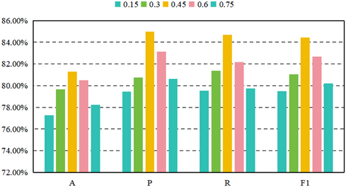
However, when $\lambda$ exceeds the optimal value of 0.45, the weight of high-order interaction features increases further, diminishing the contribution of linear features to the overall modeling. This can introduce excessive complex feature interactions or even noise, causing the model to lose its ability to effectively represent global features. Additionally, too many high-order features may amplify irrelevant patterns in the transformer data, leading to a decrease in the model's ability to identify key fault patterns. Thus, it is evident that a balance between linear features and high-order interaction features is essential for diagnostic tasks. When $\lambda =0.45$ , it strikes the optimal balance between global trend modeling and high-order feature representation, allowing the model to effectively and efficiently capture complex fault patterns. This balance not only underscores the importance of $\lambda$ but also highlights the critical role of well-designed high-order interactions in improving diagnostic performance.

4.5.4 The Impact of Different $N$ Values on Classification Results

To further investigate the impact of different numbers of AHOHN layers on fault data, we conducted experiments with $N$ values set to 1, 3, 5, 7, 9, and 11, as shown in Figure 6.

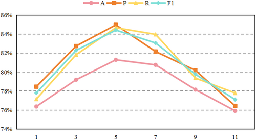
The results show that as $N$ increases from 1 to 5, the model's performance gradually improves. This is because a shallower network can only capture basic local features and is insufficient for fully extracting complex temporal dynamics and nonlinear feature interactions. As the number of layers increases, the model benefits from a layered structure and mixed attention mechanisms, allowing it to better integrate temporal information and the correlations between features. The high-order feature enhancement module also captures the nonlinear relationships in the data more effectively, significantly boosting the model's diagnostic capabilities.

However, when the number of layers exceeds 5, model performance starts to decline. This is primarily due to the high network complexity, which leads to feature redundancy and noise amplification, diluting the expression of key features. Additionally, the increased number of parameters complicates optimization, potentially causing the model to fall into local optima. A deeper network is also more prone to overfitting the detailed features of the training data, rather than general patterns, which reduces robustness on the test set. In summary, when N is set to 5, the model achieves the optimal balance between feature extraction capability and complexity. It can effectively capture the complex features in transformer fault data while avoiding issues such as feature redundancy and overfitting.

5 Conclusion

Transformer fault diagnosis is critical for the safe and stable operation of power systems, as it enables rapid and accurate fault type identification, guiding maintenance operations effectively. Traditional methods struggle with multi-scale temporal feature extraction and high-order feature representation, limiting their ability to handle complex dynamic data. To address this, we propose the MSTAFN. The MSTAFN model generates time-position vectors using a temporal information encoding module and then fuses these vectors with transformer data features through the AHOHN module, capturing temporal change characteristics. It also enhances high-order feature expression and captures complex nonlinear relationships between features, improving the model's ability to understand and model the data. The MSTF module dynamically adjusts the fusion ratio of multi-scale temporal features and global dependencies, ensuring adaptability to different tasks and data distributions. By integrating various feature information, MSTAFN achieves accurate transformer fault classification, significantly improving diagnostic accuracy. In the future, we plan to optimize the model for more complex environments, focusing on challenges such as missing data, noise, and real-time performance, while exploring its application in diagnosing faults in other power equipment to enhance the safety and efficiency of power systems.

Author Contributions

XuMing Liu: conceptualization. XiaoKun He: data curation. YongLin Li: methodology.

Ethics Statement

This research does not involve any human, animal, or plant experiments.

Conflicts of Interest

The authors declare no conflicts of interest.

Open Research

Data Availability Statement

The data that support the findings of this study are available from the corresponding author upon reasonable request.

References

1Z. Xing and Y. He, “Multi-Modal Information Analysis for Fault Diagnosis With Time-Series Data From Power Transformer,” International Journal of Electrical Power & Energy Systems 144 (2023): 108567.
10.1016/j.ijepes.2022.108567
Web of Science® Google Scholar
2Z. Wu, L. Zhou, T. Lin, et al., “A New Testing Method for the Diagnosis of Winding Faults in Transformer,” IEEE Transactions on Instrumentation and Measurement 69, no. 11 (2020): 9203–9214.
10.1109/TIM.2020.2998877
CAS Web of Science® Google Scholar
3S. Pramanik, A. Ganesh, and V. C. Duvvury, “Double-End Excitation of a Single Isolated Transformer Winding: An Improved Frequency Response Analysis for Fault Detection,” IEEE Transactions on Power Delivery 37, no. 1 (2021): 619–626.
10.1109/TPWRD.2021.3067863
Google Scholar
4A. Palani, S. Santhi, S. Gopalakrishna, and V. Jayashankar, “Real-Time Techniques to Measure Winding Displacement in Transformers During Short-Circuit Tests,” IEEE Transactions on Power Delivery 23, no. 2 (2008): 726–732.
10.1109/TPWRD.2007.911110
Web of Science® Google Scholar
5J. Christian and K. Feser, “Procedures for Detecting Winding Displacements in Power Transformers by the Transfer Function Method,” IEEE Transactions on Power Delivery 19, no. 1 (2004): 214–220.
10.1109/TPWRD.2003.820221
Web of Science® Google Scholar
6S. Mortazavian, M. M. Shabestary, Y. A. R. I. Mohamed, and G. B. Gharehpetian, “Experimental Studies on Monitoring and Metering of Radial Deformations on Transformer HV Winding Using Image Processing and UWB Transceivers,” IEEE Transactions on Industrial Informatics 11, no. 6 (2015): 1334–1345.
10.1109/TII.2015.2479582
Web of Science® Google Scholar
7M. Demirci, H. Gözde, and M. C. Taplamacioglu, “Improvement of Power Transformer Fault Diagnosis by Using Sequential Kalman Filter Sensor Fusion,” International Journal of Electrical Power & Energy Systems 149 (2023): 109038.
10.1016/j.ijepes.2023.109038
Web of Science® Google Scholar
8J. I. Aizpurua, V. M. Catterson, B. G. Stewart, et al., “Power Transformer Dissolved Gas Analysis Through Bayesian Networks and Hypothesis Testing,” IEEE Transactions on Dielectrics and Electrical Insulation 25, no. 2 (2018): 494–506.
10.1109/TDEI.2018.006766
CAS Web of Science® Google Scholar
9S. Lu, W. Gao, C. Hong, and Y. Sun, “A Newly-Designed Fault Diagnostic Method for Transformers via Improved Empirical Wavelet Transform and Kernel Extreme Learning Machine,” Advanced Engineering Informatics 49 (2021): 101320.
10.1016/j.aei.2021.101320
Web of Science® Google Scholar
10X. Zhao, M. Jia, and Z. Liu, “Semisupervised Graph Convolution Deep Belief Network for Fault Diagnosis of Electormechanical System With Limited Labeled Data,” IEEE Transactions on Industrial Informatics 17, no. 8 (2020): 5450–5460.
10.1109/TII.2020.3034189
Google Scholar
11H. Liu, H. Zhao, J. Wang, S. Yuan, and W. Feng, “LSTM-GAN-AE: A Promising Approach for Fault Diagnosis in Machine Health Monitoring,” IEEE Transactions on Instrumentation and Measurement 71 (2021): 1–13.
Google Scholar
12N. A. Tunio, A. A. Hashmani, S. Khokhar, M. A. Tunio, and M. Faheem, “Fault Detection and Classification in Overhead Transmission Lines Through Comprehensive Feature Extraction Using Temporal Convolution Neural Network,” Engineering Reports 6, no. 12 (2024): e12950, https://doi.org/10.1002/eng2.12950.
10.1002/eng2.12950
Web of Science® Google Scholar
13K. He, X. Zhang, S. Ren, and J. Sun, “Deep Residual Learning for Image Recognition,” Proceedings of the IEEE Conference on Computer Vision and Pattern Recognition (2016): 770–778.
Google Scholar
14S. Zhang, R. Wang, L. Wang, Y. Si, A. Lin, and Y. Wang, “Fault Diagnosis for Power Converters Based on Incremental Learning,” IEEE Transactions on Instrumentation and Measurement 72 (2023): 1–13.
PubMed Web of Science® Google Scholar
15Z. Xing, Y. He, and W. Zhang, “An Online Multiple Open-Switch Fault Diagnosis Method for T-Type Three-Level Inverters Based on Multimodal Deep Residual Filter Network,” IEEE Transactions on Industrial Electronics 70, no. 10 (2022): 10669–10679.
10.1109/TIE.2022.3222663
Google Scholar
16H. Xiong, Z. Wang, G. Wu, Y. Pan, Z. Yang, and Z. Long, “Steering Actuator Fault Diagnosis for Autonomous Vehicle With an Adaptive Denoising Residual Network,” IEEE Transactions on Instrumentation and Measurement 71 (2022): 1–13.
Web of Science® Google Scholar
17E. W. Gituku, J. K. Kimotho, and J. G. Njiri, “Cross-Domain Bearing Fault Diagnosis With Refined Composite Multiscale Fuzzy Entropy and the Self-Organizing Fuzzy Classifier,” Engineering Reports 3, no. 3 (2021): e12307.
10.1002/eng2.12307
Web of Science® Google Scholar
18R. Liu, F. Wang, B. Yang, and S. J. Qin, “Multiscale Kernel-Based Residual Convolutional Neural Network for Motor Fault Diagnosis Under Nonstationary Conditions,” IEEE Transactions on Industrial Informatics 16, no. 6 (2019): 3797–3806.
10.1109/TII.2019.2941868
Google Scholar
19X. Li, H. Hu, S. Zhang, and G. Tang, “A Fault Diagnosis Method for Rotating Machinery With Semi-Supervised Graph Convolutional Network and Images Converted From Vibration Signals,” IEEE Sensors Journal 23, no. 11 (2023): 11946–11955.
10.1109/JSEN.2023.3267427
Web of Science® Google Scholar
20W. Liao, D. Yang, Y. Wang, and X. Ren, “Fault Diagnosis of Power Transformers Using Graph Convolutional Network,” CSEE Journal of Power and Energy Systems 7, no. 2 (2020): 241–249.
Web of Science® Google Scholar
21L. Liu, B. Wang, F. Ma, et al., “A Concurrent Fault Diagnosis Method of Transformer Based on Graph Convolutional Network and Knowledge Graph,” Frontiers in Energy Research 10 (2022): 837553.
10.3389/fenrg.2022.837553
Web of Science® Google Scholar
22Y. Zhou, Y. He, Z. Xing, et al., “Vibration Signal-Based Fusion Residual Attention Model for Power Transformer Fault Diagnosis,” IEEE Sensors Journal 24, no. 10 (2024): 17231–17242, https://doi.org/10.1109/JSEN.2024.3382811.
10.1109/JSEN.2024.3382811
CAS Web of Science® Google Scholar
23Y. Ding, M. Jia, Q. Miao, and Y. Cao, “A Novel Time–Frequency Transformer Based on Self–Attention Mechanism and Its Application in Fault Diagnosis of Rolling Bearings,” Mechanical Systems and Signal Processing 168 (2022): 108616.
10.1016/j.ymssp.2021.108616
Web of Science® Google Scholar
24G. Zhou, C. Sun, H. Xu, Z. Zhou, X. Jiang, and Y. Wang, “ A Transformer Fault Diagnosis Method Based on Convolutional Neural Networks With Channel Attention Mechanism and Data Augmentation,” in The Proceedings of the 11th Frontier Academic Forum of Electrical Engineering (FAFEE2024), vol. 1287, ed. Q. Yang and J. Li (Springer, 2025), 480–487.
Google Scholar
25H. Wang, J. Xu, R. Yan, and R. X. Gao, “A New Intelligent Bearing Fault Diagnosis Method Using SDP Representation and SE-CNN,” IEEE Transactions on Instrumentation and Measurement 69, no. 5 (2019): 2377–2389.
10.1109/TIM.2019.2956332
Google Scholar
26K. Hong, M. Jin, and H. Huang, “Transformer Winding Fault Diagnosis Using Vibration Image and Deep Learning,” IEEE Transactions on Power Delivery 36, no. 2 (2020): 676–685.
10.1109/TPWRD.2020.2988820
Google Scholar
27J. Yin, X. Zhou, Y. Ma, Y. Wu, and X. Xu, “ Power Transformer Fault Diagnosis Based on Multi-Class Multi-Kernel Learning Relevance Vector Machine,” in 2015 IEEE International Conference on Mechatronics and Automation (ICMA) (IEEE, 2015), 217–221.
10.1109/ICMA.2015.7237485
Google Scholar
28E. Li, L. Wang, and B. Song, “Fault Diagnosis of Power Transformers With Membership Degree,” IEEE Access 7 (2019): 28791–28798.
10.1109/ACCESS.2019.2902299
Web of Science® Google Scholar
29K. Chatterjee, S. Dawn, V. K. Jadoun, and R. K. Jarial, “Novel Prediction-Reliability Based Graphical DGA Technique Using Multi-Layer Perceptron Network & Gas Ratio Combination Algorithm,” IET Science, Measurement & Technology 13, no. 6 (2019): 836–842.
10.1049/iet-smt.2018.5397
Web of Science® Google Scholar
30N. Li, B. Li, and L. Gao, “Transient Stability Assessment of Power System Based on XGBoost and Factorization Machine,” IEEE Access 8 (2020): 28403–28414.
10.1109/ACCESS.2020.2969446
Web of Science® Google Scholar
31L. Hong, Z. Chen, Y. Wang, M. Shahidehpour, and M. Wu, “A Novel SVM-Based Decision Framework Considering Feature Distribution for Power Transformer Fault Diagnosis,” Energy Reports 8 (2022): 9392–9401.
10.1016/j.egyr.2022.07.062
Web of Science® Google Scholar
32O. Kherif, Y. Benmahamed, M. Teguar, A. Boubakeur, and S. S. Ghoneim, “Accuracy Improvement of Power Transformer Faults Diagnostic Using KNN Classifier With Decision Tree Principle,” IEEE Access 9 (2021): 81693–81701, https://doi.org/10.1109/ACCESS.2021.3086135.
10.1109/ACCESS.2021.3086135
Web of Science® Google Scholar
33B. Zhang, F. Jiao, J. Tong, Y. Tan, Z. Zhang, and S. Lin, “Muti-Branch Residual Multiscale CNN Based Power Transformer Fault Diagnosis on Vibration Signal,” CSEE Journal of Power and Energy Systems (2023), https://doi.org/10.17775/CSEEJPES.2022.00490.
10.17775/CSEEJPES.2022.00490
Google Scholar
34L. Li, S. Wang, Y. Zhao, and F. Wang, “ Fault Diagnosis for Single-Phase Grounding in Distribution Network Based on Hilbert-Huang Transform and Siamese Convolution Neural Network,” in 2023 35th Chinese Control and Decision Conference (CCDC) (IEEE, 2023), 3571–3576.
10.1109/CCDC58219.2023.10326495
Google Scholar

Volume7, Issue5

May 2025

e70152

A Multi-Scale Time Adaptive Fusion Network for Transformer Fault Diagnosis

ABSTRACT

1 Introduction

2 Related Work

2.1 Diagnosis Method Based on Physical Principles

2.2 Diagnosis Methods Based on Machine Learning

2.3 Hybrid Diagnostic Model Based on Deep Learning

3 Methods

3.1 Temporal Information Encoding

3.2 Adaptive High-Order Hybrid Network

3.2.1 Hybrid Attention

3.2.2 High-Order Feature Enhancement

3.2.3 Adaptive Feature Reconstruction

3.3 Multi-Scale Temporal Feature Fusion

3.3.1 BIGRU Model

3.3.2 MSMRN Model

3.3.3 Adaptive Temporal Fusion

3.4 Classifier

4 Experiments and Result Analysis

4.1 Dataset

4.2 Experimental Setup

4.3 Loss Function

4.4 Evaluation Metrics

4.5 Results and Analysis

4.5.1 Comparative Experiments

4.5.2 Ablation Study

4.5.3 The Impact of Different λ $$ \lambda $$ Values on Classification Results

4.5.4 The Impact of Different N $$ N $$ Values on Classification Results

5 Conclusion

Author Contributions

Ethics Statement

Conflicts of Interest

Open Research

Data Availability Statement

References

Figures

References

Related

Information

4.5.3 The Impact of Different $\lambda$ Values on Classification Results

4.5.4 The Impact of Different $N$ Values on Classification Results