Random Walk-Based GOOSE Algorithm for Solving Engineering Structural Design Problems
Funding: The authors received no specific funding for this work.
ABSTRACT
The proposed Random Walk-based Improved GOOSE (IGOOSE) search algorithm is a novel population-based meta-heuristic algorithm inspired by the collective movement patterns of geese and the stochastic nature of random walks. This algorithm includes the inherent balance between exploration and exploitation by integrating random walk behavior with local search strategies. In this paper, the IGOOSE search algorithm has been rigorously tested across 23 benchmark functions where 13 benchmarks are with varying dimensions (10, 30, 50, and 100 dimensions). These benchmarks provide a diverse range of optimization landscapes, enabling comprehensive evaluation of IGOOSE algorithm performance under different problem complexities. The algorithm is tested by various parameters such as convergence speed, magnitude of solution, and robustness for different dimensions. Further, IGOOSE algorithm is applied to optimize eight distinct engineering problems, showcasing its versatility and effectiveness in real-world scenarios. The results of these evaluations highlight IGOOSE algorithm as a competitive optimization tool, offering promising performance across both standard benchmarks and complex structural engineering problems. Its ability to balance exploration and exploitation effectively, combined with its ability to deal with different problems, positions IGOOSE algorithm as a valuable tool.
1 Introduction
Meta-heuristic algorithms (MAs) have undergone rapid development in recent years. They integrate stochastic and local search algorithms and are extensively employed to address global optimization challenges across various domains. Compared to traditional algorithms, MAs excel in handling complex, multimodal, noncontinuous, and nondifferentiable real-world problems due to their incorporation of random elements [1]. For example, MAs can be used to solve problems in clustering [2], shape optimization [3], image processing [4], deep learning [5], machine learning [6], path planning [7], engineering problems [8], and other domains. MAs emulate the behavior of humans or animals and utilize principles from physics and chemistry to formulate mathematical models for optimization algorithms. As a result, MAs are categorized into four types: evolution-based algorithms, human-based algorithms, physics-based algorithms, and swarm-based intelligence algorithms [9]. Evolution-based algorithms improve successive generations by emulating Darwin's principles of natural selection, promoting collective progress within populations and few of them are Barnacles Mating Optimizer [10], Partial reinforcement optimizer [11], Differential Evolution [12], and Cultural evolution algorithm [13]. Human-based algorithms draw inspiration from various social behaviors such as teaching, learning, competition, and cooperation observed in human societies, and a few of them are Driving Training-Based Optimization [14], Human urbanization algorithm [15], Preschool Education Optimization Algorithm [16], Dollmaker Optimization Algorithm [17], and Hiking Optimization Algorithm [18]. Algorithms based on physics derive inspiration from principles and experiments in these scientific disciplines examples of them are Propagation Search Algorithm [19], Prism refraction search [20], Kepler optimization algorithm [21], and Equilibrium optimizer [22]. Swarm-based intelligence algorithms aim to find optimal solutions by simulating group behaviors and leveraging collective intelligence, and the examples are Stochastic Shaking Algorithm [23], Cock-Hen-Chicken Optimizer [24], Elk herd optimizer [25], The Pine Cone Optimization Algorithm [26], and giant pacific octopus optimizer [27]. In Table 1, different algorithms mentioned in the literature demonstrate strong capabilities in global search and effectively handle continuous optimization problems.
| Ref | Algorithm name | Research gaps |
|---|---|---|
| [10] | Barnacles Mating Optimizer (BMO) | Lack of extensive comparative studies with other evolutionary algorithms |
| [11] | Partial Reinforcement Optimizer (PRO) | Limited exploration of reinforcement learning strategies for optimization |
| [12] | Differential Evolution (DE) | Facing challenges in handling high-dimensional optimization problems efficiently |
| [13] | Cultural evolution algorithm (CEO) | Limited application and validation in diverse optimization domains |
| [14] | Driving Training-Based Optimization (DTBO) | Need to validate on scalability and robustness in solving complex optimization problems |
| [15] | Human Urbanization Algorithm (HUA) | Lack of comprehensive benchmarking against other urban-inspired algorithms |
| [16] | Preschool Education Optimization Algorithm (PEOA) | Limited exploration of educational theories in algorithm design and optimization |
| [17] | Dollmaker Optimization Algorithm (DOA) | Lack of studies on the algorithm's adaptability across different problem domains |
| [18] | Hiking Optimization Algorithm (HOA) | Need to rigorous testing on large-scale optimization problems and performance comparison |
| [19] | Propagation Search Algorithm (PSA) | Facing challenges in optimizing problems with high computational complexity |
| [20] | Prism Refraction Search (PRS) | Limited studies on the algorithm's convergence properties and parameter sensitivity |
| [21] | Kepler Optimization Algorithm (KOA) | Need to validate real-world engineering and scientific applications |
| [22] | Equilibrium Optimizer (EO) | Lack of comprehensive analysis on algorithm convergence and solution quality |
| [23] | Stochastic Shaking Algorithm (SSOA) | Limited exploration of the algorithm's performance on various optimization benchmarks |
| [24] | Cock-Hen-Chicken Optimizer (CHCO) | Need to do comparative studies with other nature-inspired algorithms in optimization tasks |
| [25] | Elk Herd Optimizer (EHO) | Facing challenges in handling dynamic optimization problems and adaptation rates |
| [26] | Pine Cone Optimization Algorithm (PCOA) | Lack of studies on algorithm scalability and efficiency in high-dimensional spaces |
| [27] | Giant Pacific Octopus Optimizer (GPO) | Limited validation on diverse engineering and real-world applications. |
| [28] | GOOSE algorithm | Limited exploration on real-world engineering problems and potential for further performance improvement and comparative analysis with other metaheuristic algorithms |
| [29] | Teaching-Learning-Based Optimization (TLBO) | Needs enhanced diversity mechanisms and further validation on more diverse and complex optimization problems |
| [30] | Whale Optimization Algorithm (WOA) | Requires improvement in balancing exploration and exploitation, and needs to be tested on more diverse problem sets |
| [31] | Gravitational Search Algorithm (GSA) | Issues with slow convergence and premature convergence, and lacks extensive comparative studies with newer algorithms |
| [32] | White Shark Optimizer (WSO) | Limited applications to specific types of optimization problems and needs more comparative studies to establish robustness |
| [33] | Gray Wolf Optimizer (GWO) | Struggles with maintaining diversity in the population and may require hybridization with other algorithms to improve performance |
| [34] | Marine Predators Algorithm (MPA) | Needs further analysis on complex and high-dimensional problems, and comparative studies with other recent algorithms |
| [35] | Tunicate Swarm Algorithm (TSA) | Requires further testing on large-scale and real-world problems and optimization of parameter settings |
| [36] | Multi-Verse Optimizer (MVO) | Limited handling of multimodal problems and requires enhancements in exploration mechanisms |
| [37] | Ant Lion Optimizer (ALO) | Struggle with exploitation in complex multimodal problems and needs to improve its balance between exploration and exploitation, particularly in high-dimensional spaces |
| [38] | Harris Hawks Optimization (HHO) | Its convergence speed and solution accuracy can be improved and the performance in dynamic environments has not been thoroughly explored |
| [39] | Sine Cosine Algorithm (SCA) | Its convergence to local optima remains an issue and enhancement is required to increase its robustness across a wider range of problems |
| [40] | Moth-Flame Optimization (MFO) | Exhibits premature convergence in some scenarios and needed to improve its performance in complex optimization landscapes |
| [41] | Arithmetic Optimization Algorithm (AOA) | Its scalability to very high-dimensional problems is not well-studied |
| [42] | Slime Mold Algorithm (SMA) | Its performance in highly dynamic or noisy environments is underexplored and needs to fine-tune its parameters for improved convergence efficiency. |
| [43] | Archimedes Optimization Algorithm (AROA) | Requires further investigation into its performance on large-scale and complex optimization problems. |
| [44] | Aquila Optimizer (AO) | Its long-term convergence behavior and performance on highly multimodal functions require more extensive validation |
| [45] | Henry Gas Solubility Optimizer (HGS) | Its application to real-world problems and its scalability need further study |
| [46] | Rabbit optimizer (RO) | Its scalability to very high-dimensional problems is not well-studied |
| [47] | Hummingbird algorithm (HA) | Its performance showed the premature convergence in certain cases |
| [48] | Cooperative strategy-based differential evolution algorithm (CSDEA) | Requires further investigation into its performance on large-scale and complex optimization problems |
| [49] | Quick crisscross sine cosine algorithm (QCSCA) | Requires further investigation into its performance on large-scale and complex optimization problems. |
| [50] | Modified Whale optimization algorithm (MWOA) | Exhibits premature convergence in some scenarios and needs to improve its performance in complex optimization landscapes |
However, they face significant challenges when applied to solving discrete optimization problems. The classical GOOSE algorithm, developed by Hamad and Rashid [28] in 2024, inspired from collective behavior of geese to optimization problems. Inspired by the synchronized movements and effective navigation strategies of geese, classical GOOSE harnesses cooperative search techniques among individual solutions to explore and exploit the solution of space efficiently. Several investigations have demonstrated that the GOOSE method is effective at addressing optimization challenges [28]. However, as real-world problems grow in complexity, the original GOOSE algorithm struggles to effectively address these challenges and deliver satisfactory results. There is a clear need for enhancements to improve its efficacy.
This paper introduces an improved IGOOSE (IGOOSE) algorithm, which uses a random walk strategy to enhance convergence speed and reduce the risk of getting stuck in local optima. In this work, the CEC benchmark test functions are validated, among them 13 benchmarks were validated for different dimensions (10D, 30D, 50D, and 100D), and 8 engineering structural designs [51] are used to verify the superiority of IGOOSE algorithm.
2 Traditional GOOSE Algorithm
A Goose, multiple geese, Geese are waterfowls from the Anatidae family, in size, swans < Geese > ducks. They are sociable and feed on nuts, berries, plants, grass, and seeds. They spend most of their time on land and fly in a “V” shape. When the leading goose becomes tired, another takes over. Goose are loyal, lifelong mates, and protective of their families. They display grieving behavior when losing a mate or eggs and have deep feelings for their group.
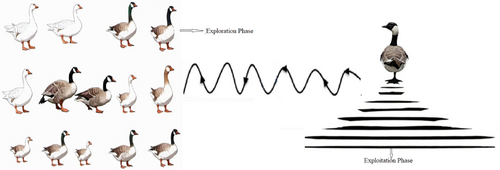
The first recorded usage of a goose for protection dates back to ancient Rome. Geese are used to protect police stations and installations in Xinjiang, while in Dumbarton, Scotland, a storehouse for Ballantine's whiskey was guarded by a gander for 53 years until modern cameras were added. Goose population in natural environments have some members serving as guardians who protect them while others forage or rest. They stand on one leg and sometimes carry a small stone to stay awake. When they hear strange sounds or movements, they make loud noises to keep the herd safe. Gooses are highly possessive of their homes, especially during mating and fledging periods. They respond to human observations in a beneficial manner, with their loud, aggressive sound being perfect for guarding the premises. Geese usually stay in groups in their shelters, with one geese assigned to guard. The sound of the rock spreads to other geese, which mimics the state of exploitation under optimization. As a result, it takes time for others to notice the guardian goose's cry. Sound flows at a speed of 343 m per second through the air therefore it requires very less time to get alert. Figure 1 depicts the GOOSE exploitation phase.
2.1 Mathematical Formulation of GOOSE
Initialize the GOOSE population as an X matrix. The goose's location is represented in X, and search agents beyond the search space are returned in the boundary after initializing the population, with fitness determined through standardized benchmark functions in each iteration. The search involves measuring the fitness of each agent within the X grid and comparing it to the fitness of the remaining agents to evaluate BestFitness and Best Position (BestX). BestFitness and BestX are operations that compare the fitness of current row (fitnessi + 1) and return the fitness of the previous row during iterations. In GOOSE algorithm, the exploitation and exploration stages are provided equal weight using a random variable termed “rnd”. A conditional phase divides iterations equally between exploration and exploitation. Variables pro, rnd., and coe (coe less than or equal to 0.17) are introduced to randomly determine the price (between 0 and 1). The pro parameter indicates which formula is valid, while the weight of the stone transported by the geese is found out. Further discussion on exploration and exploitation will follow.
2.2 Exploration Phase
The distribution of exploitation and exploration phases is determined by a random variable (rnd).
2.2.1 Exploration Phase
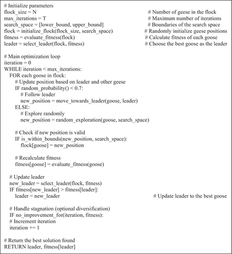
The number of problem dimensions is denoted by dim, while Best_pos represents the optimal position () found in the search area. In Figure 2, the GOOSE algorithm pseudo-code is presented.
2.3 Proposed RW-GOOSE Algorithm
In this research paper, we explore the potential drawbacks of the GOOSE algorithm and propose a hybridization strategy with a random walk approach to address these challenges. The GOOSE algorithm, while effective, can be limited by its tendency to trap in local optima, slow convergence in complex spaces, and sensitivity to initial conditions. By integrating a random walk strategy, we aim to enhance exploration capabilities, diversify search efforts, accelerate convergence, improve robustness against noise, and enhance adaptability across diverse problem domains. This hybrid approach harnesses the deterministic strengths of GOOSE alongside the stochastic nature of random walk, aiming to achieve more efficient and effective optimization outcomes in practical applications.
2.4 Random Walk
The random walk strategy enhances optimization algorithms by introducing randomness, improving exploration capabilities and preventing premature convergence to local optima. It maintains diversity in the search space, making the algorithms more robust and effective, especially in complex optimization problems.
Here, is a parametric variable that controls the step size in each iteration.
2.5 Design of Proposed Random Walk-Based GOOSE (IGOOSE) Algorithm
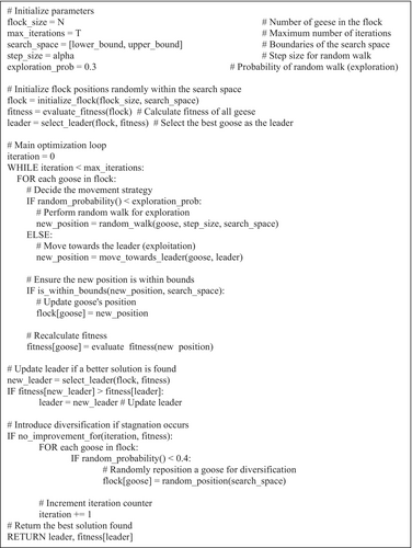
The classical GOOSE algorithm begins with an initial population of geese denoted as . Throughout each iteration, a random walk is applied exclusively to the leading individuals, , of the population. Here, a parameter vector linearly decreases from 2 to 0 as iterations advance. This algorithm integrates a random walk where step sizes are drawn from a Cauchy distribution.
The rationale for using a Cauchy distributed random step size lies in its infinite variance, allowing for occasional large jumps. This capability proves highly effective during stagnation periods, facilitating exploration of the search space by the leading geese. This exploration, in turn, helps safeguard and guide the other geese in the population. Importantly, the algorithm does not introduce additional objective function evaluations, ensuring consistency in function evaluation across both versions of the algorithm. The pseudo-code of the proposed algorithm IGOOSE algorithm is described in Figure 3.
3 Numerical Experiments
In this section, the performance of the GOOSE algorithm and the proposed IGOOSE algorithm is evaluated using the criteria of IEEE CEC benchmark functions [28]. These benchmarks encompass 23 unconstrained optimization problems of unimodal and multimodal types, with fixed dimensions and varying levels of difficulty. Among the IEEE CEC benchmark functions, 13 benchmarks were validated across different dimensions: 10, 30, 50, and 100. All numerical experiments were conducted using MATLAB 2022a.
3.1 Benchmark Functions
Each test function is executed 30 times across dimensions of 10D, 30D, 50D, and 100D to evaluate the performance of both algorithms. The initial population is uniformly generated using a random number generator. Table 2 presents the standard CEC benchmark functions.
| Functions | Dimensions | Range | fmin |
|---|---|---|---|
| 10D, 30D, 50D, 100D | [−100, 100] | 0 | |
| 10D, 30D, 50D, 100D | [−10,10] | 0 | |
| 10D, 30D, 50D, 100D | [−100, 100] | 0 | |
| 10D, 30D, 50D, 100D | [−100, 100] | 0 | |
| 10D, 30D, 50D, 100D | [−38, 38] | 0 | |
| 10D, 30D, 50D, 100D | [−100, 100] | 0 | |
| 10D, 30D, 50D, 100D | [−1.28, 1.28] | 0 | |
| 10D, 30D, 50D, 100D | [−500, 500] | −418.98295 | |
|
|
10D, 30D, 50D, 100D | [−5.12, 5.12] | 0 |
| 10D, 30D, 50D, 100D | [−32, 32] | 0 | |
| 10D, 30D, 50D, 100D | [−600, 600] | 0 | |
|
|
10D, 30D, 50D, 100D | [−50, 50] | 0 |
| 10D, 30D, 50D, 100D | [−50, 50] | 0 | |
| 2 | [−65.536, 65.536] | 1 | |
| 4 | [−5, 5] | 0.00030 | |
| 2 | [−5, 5] | −1.0316 | |
| 2 | [−5, 5] | 0.398 | |
| 2 | [−2,2] | 3 | |
| 3 | [1, 3] | −3.32 | |
| 6 | [0, 1] | −3.32 | |
| 4 | [0, 10] | −10.1532 | |
| 4 | [0, 10] | −10.4028 | |
| 4 | [0, 10] | −10.5363 |
3.2 Analysis of the Results
All the results represented in this research paper address the format specified by the IEEE CEC [66]. Tables 3, 5, and 6 display the outcomes of applying the GOOSE algorithm and IGOOSE algorithm on IEEE CEC test functions for 10, 50, and 100 dimensions, as detailed in the computational formulas of IEEE CEC functions F1–F13 in Table 2. Table 3 presents the 10-dimensional search outcomes for the proposed IGOOSE and GOOSE algorithms. Table 4 presents the results of 23 IEEE CEC tests conducted for 30 dimensions, also based on the computational formulas in Table 2. These tables report the maximum, minimum, mean, median, and standard deviation of the absolute error values of the objective function for the test functions. Since unimodal problems (F1-F7, suitable for evaluating the exploitation capability of any search algorithm), multimodal problems (F8-F13, the multimodal test problem typically evaluates the search algorithm's exploration strength and local optima avoidance ability), and fixed dimensional problems (F14-F23, suitable for any high-dimensional and hybrid complex problems) are in the IEEE CEC benchmark problem set. From Tables 2, 4–6, it is evident that IGOOSE algorithm outperforms the GOOSE algorithm across all statistical measures. Therefore, in terms of exploiting the search regions around the explored areas, IGOOSE algorithm is superior to the GOOSE algorithm.
| IGOOSE | GOOSE | |||||||||
|---|---|---|---|---|---|---|---|---|---|---|
| Avg | Std | Best | Worst | Median | Avg | Std | Best | Worst | Median | |
| F1 | 5.63E-05 | 4.26E-05 | 2.53E-05 | 0.000131 | 3.85E-05 | 3.6E-05 | 2.05E-05 | 1.26E-05 | 6.26E-05 | 2.73E-05 |
| F2 | 0.015331 | 0.002782 | 0.011957 | 0.018655 | 0.016053 | 0.020684 | 0.009114 | 0.012942 | 0.035561 | 0.01814 |
| F3 | 97.66608 | 173.5325 | 7.49E-05 | 400.5529 | 0.000583 | 242.1433 | 171.1426 | 0.000226 | 404.4416 | 325.9187 |
| F4 | 7.881002 | 13.01657 | 0.003393 | 30.00262 | 0.007121 | 3.932929 | 3.820431 | 0.003633 | 8.667514 | 5.140625 |
| F5 | 35.03801 | 65.10406 | 2.142237 | 151.4315 | 7.062609 | 7.77E-05 | 3.7E-05 | 4.95E-05 | 0.000141 | 6.36E-05 |
| F6 | 6.41E-05 | 2.82E-05 | 4.56E-05 | 0.000114 | 5.36E-05 | 7.77E-05 | 3.7E-05 | 4.95E-05 | 0.000141 | 6.36E-05 |
| F7 | 0.00839 | 0.005595 | 0.003759 | 0.014624 | 0.004994 | 0.008602 | 0.004635 | 0.001936 | 0.014049 | 0.008115 |
| F8 | −2806.62 | 385.4139 | −3143.59 | −2155.05 | −2960.51 | −2685.29 | 361.5436 | −3084.27 | −2334.2 | −2531.64 |
| F9 | 33.43902 | 11.74125 | 16.92629 | 46.76862 | 33.83199 | 43.98678 | 13.78948 | 24.88661 | 63.67949 | 43.78445 |
| F10 | 6.522736 | 6.819754 | 0.020932 | 18.05964 | 4.499182 | 14.82505 | 8.305398 | 0.005842 | 19.49275 | 18.34157 |
| F11 | 33.85018 | 47.44767 | 1.7E-06 | 100.1212 | 0.481951 | 98.31139 | 25.13554 | 63.21026 | 128.4562 | 104.0645 |
| F12 | 8.591365 | 11.45327 | 1.507135 | 28.17418 | 2.207285 | 11.86392 | 14.45159 | 0.648454 | 32.10024 | 3.226769 |
| F13 | 2.94E-05 | 5.3E-06 | 2.13E-05 | 3.45E-05 | 2.95E-05 | 2.52E-05 | 1.18E-05 | 8.64E-06 | 3.92E-05 | 2.32E-05 |
| Functions | Parameters | IGOOSE | GOOSE [28] | TLBO [29] | WOA [30] | GSA [31] | WSO [32] | GWO [33] | MPA [34] | TSA [35] | MVO [36] |
|---|---|---|---|---|---|---|---|---|---|---|---|
| F1 | Mean | 25.42282 | 290.6142 | 9.04E-75 | 5.80E-155 | 1.15E-16 | 323.1097 | 4.55E-59 | 9.29E-50 | 3.20E-47 | 0.151165 |
| Best | 0.009773 | 0.007816 | 3.06E-77 | 6.00E-167 | 4.90E-17 | 72.27965 | 1.72E-60 | 7.49E-52 | 1.71E-49 | 0.099666 | |
| Worst | 112.353 | 1453.02 | 7.49E-74 | 6.00E-154 | 3.20E-16 | 901.2379 | 3.48E-58 | 6.72E-49 | 2.09E-46 | 0.247637 | |
| Std | 49.0109 | 649.8043 | 2.06E-74 | 1.60E-154 | 6.07E-17 | 238.7674 | 8.56E-59 | 1.88E-49 | 6.32E-47 | 0.042235 | |
| Median | 0.018009 | 0.01451 | 8.83E-76 | 7.00E-161 | 1.04E-16 | 282.8347 | 1.94E-59 | 2.03E-50 | 3.66E-48 | 0.135998 | |
| F2 | Mean | 98.61287 | 135.2225 | 1.06E-38 | 6.40E-104 | 5.37E-08 | 3.776208 | 1.64E-34 | 1.04E-27 | 1.90E-28 | 0.26047 |
| Best | 67.17263 | 56.32044 | 2.62E-40 | 1.90E-114 | 3.07E-08 | 0.756212 | 7.38E-36 | 5.61E-30 | 1.02E-30 | 0.179542 | |
| Worst | 140.0143 | 195.715 | 8.43E-38 | 1.20E-102 | 9.17E-08 | 8.958666 | 6.42E-34 | 3.43E-27 | 2.01E-27 | 0.434829 | |
| Std | 31.68491 | 54.90727 | 1.94E-38 | 2.70E-103 | 1.56E-08 | 2.044082 | 2.04E-34 | 1.21E-27 | 4.90E-28 | 0.070258 | |
| Median | 97.9979 | 156.9493 | 3.90E-39 | 3.40E-108 | 5.17E-08 | 3.136077 | 7.85E-35 | 6.28E-28 | 2.46E-29 | 0.24991 | |
| F3 | Mean | 2928.167 | 6545.999 | 3.18E-25 | 22123.03 | 499.7092 | 2636.013 | 2.41E-14 | 1.33E-11 | 2.30E-11 | 14.63423 |
| Best | 0.935229 | 3432.186 | 1.81E-29 | 5630.916 | 182.4369 | 1088.637 | 1.58E-19 | 2.94E-20 | 8.92E-21 | 6.012495 | |
| Worst | 9445.972 | 11679.73 | 3.35E-24 | 45040.6 | 771.4986 | 5234.592 | 3.46E-13 | 2.04E-10 | 3.05E-10 | 26.20651 | |
| Std | 3874.279 | 3615.259 | 8.70E-25 | 9979.735 | 148.1048 | 1107.562 | 7.92E-14 | 4.56E-11 | 6.88E-11 | 5.595845 | |
| Median | 1931.562 | 4964.671 | 8.95E-27 | 20656.93 | 467.5755 | 2473.189 | 4.69E-16 | 1.68E-14 | 1.47E-14 | 11.89704 | |
| F4 | Mean | 2.949959 | 26.04324 | 2.74E-30 | 39.92337 | 1.277679 | 23.45023 | 1.98E-14 | 2.45E-19 | 0.00841 | 0.589797 |
| Best | 0.132737 | 0.21798 | 2.80E-31 | 0.10012 | 1.51E-08 | 18.2143 | 8.70E-16 | 5.06E-20 | 5.99E-05 | 0.230471 | |
| Worst | 4.607789 | 49.11394 | 1.45E-29 | 84.62575 | 4.579257 | 29.70858 | 1.31E-13 | 7.36E-19 | 0.039162 | 0.978307 | |
| Std | 1.67005 | 23.06187 | 3.30E-30 | 30.0497 | 1.120839 | 3.863479 | 3.05E-14 | 1.84E-19 | 0.010586 | 0.190986 | |
| Median | 3.39503 | 34.93982 | 1.68E-30 | 38.0023 | 0.992464 | 23.18626 | 8.45E-15 | 1.93E-19 | 0.003723 | 0.614103 | |
| F5 | Mean | 458.089 | 611.9825 | 26.85244 | 27.19269 | 31.08724 | 28398.06 | 26.68578 | 23.40807 | 28.60948 | 456.4057 |
| Best | 28.74255 | 28.40965 | 25.62028 | 26.43629 | 25.42943 | 2267.064 | 25.24989 | 22.82986 | 27.91037 | 27.96275 | |
| Worst | 1633.011 | 2704.292 | 28.74462 | 28.73292 | 91.45478 | 109106.7 | 28.51931 | 24.03788 | 29.46094 | 2504.324 | |
| Std | 697.0829 | 1171.323 | 0.850991 | 0.604601 | 15.68442 | 31180.39 | 0.826454 | 0.393641 | 0.450018 | 673.5282 | |
| Median | 30.17116 | 124.3583 | 26.7838 | 26.96467 | 26.31103 | 20920.32 | 26.21564 | 23.35764 | 28.8377 | 132.3027 | |
| F6 | Mean | 0.011744 | 0.012408 | 1.24652 | 0.065683 | 1.30E-16 | 343.063 | 0.721085 | 1.54E-09 | 3.719839 | 0.155721 |
| Best | 0.007708 | 0.00547 | 0.72013 | 0.009389 | 6.32E-17 | 57.61476 | 2.88E-05 | 6.22E-10 | 2.816758 | 0.108064 | |
| Worst | 0.015338 | 0.018475 | 1.934547 | 0.372513 | 3.27E-16 | 1155.801 | 1.254424 | 3.49E-09 | 4.55303 | 0.211356 | |
| Std | 0.00306 | 0.0054 | 0.307855 | 0.088652 | 5.98E-17 | 308.0894 | 0.345344 | 8.01E-10 | 0.511655 | 0.032372 | |
| Median | 0.012165 | 0.014136 | 1.183863 | 0.033701 | 1.13E-16 | 265.7647 | 0.743237 | 1.31E-09 | 3.796628 | 0.148686 | |
| F7 | Mean | 0.071642 | 0.179521 | 0.00154 | 0.001871 | 0.058546 | 9.35E-05 | 0.000789 | 0.000767 | 0.004149 | 0.012721 |
| Best | 0.030757 | 0.109318 | 0.000295 | 5.32E-05 | 0.025667 | 1.53E-06 | 0.000353 | 0.000334 | 0.0021 | 0.005047 | |
| Worst | 0.098775 | 0.3009 | 0.003987 | 0.008107 | 0.089886 | 0.000396 | 0.001578 | 0.001661 | 0.007804 | 0.0263 | |
| Std | 0.025219 | 0.080824 | 0.001198 | 0.002254 | 0.020316 | 0.000108 | 0.000346 | 0.000444 | 0.001679 | 0.005127 | |
| Median | 0.07555 | 0.13246 | 0.001089 | 0.001069 | 0.061168 | 6.40E-05 | 0.000757 | 0.000582 | 0.003973 | 0.011738 | |
| F8 | Mean | −6974.33 | −7435.47 | −5485.59 | −11384.8 | −2655.59 | −6585.34 | −6026.15 | −9607.07 | −6149.15 | −7831.31 |
| Best | −8014.06 | −7990.73 | −6913.77 | −12568.7 | −3460.74 | −8082.13 | −7136.57 | −10195.9 | −7589.76 | −8752.78 | |
| Worst | −5876.73 | −6219.19 | −4764.14 | −8654.92 | −2191.52 | −5339.49 | −4398.37 | −8487.95 | −5152.22 | −6960.7 | |
| Std | 992.8231 | 698.2076 | 559.5748 | 1421.809 | 315.5151 | 717.4584 | 694.8304 | 442.981 | 618.3085 | 496.9466 | |
| Median | −7058.56 | −7633.57 | −5491.83 | −11960.3 | −2619.13 | −6553.85 | −5799.57 | −9575.73 | −6058.25 | −7846.27 | |
| F9 | Mean | 150.681 | 154.1387 | 0 | 2.84E-15 | 2.45E+01 | 33.71054 | 8.53E-15 | 0 | 1.65E+02 | 113.0038 |
| Best | 88.42502 | 124.2656 | 0 | 0 | 15.91933 | 19.32847 | 0 | 0 | 9.94E+01 | 64.7574 | |
| Worst | 225.6012 | 184.0281 | 0 | 5.68E-14 | 4.18E+01 | 60.08227 | 5.68E-14 | 0 | 2.23E+02 | 159.2712 | |
| Std | 53.77779 | 23.0601 | 0 | 1.27E-14 | 6.72E+00 | 11.24004 | 2.08E-14 | 0 | 3.24E+01 | 29.65035 | |
| Median | 144.8089 | 156.8133 | 0 | 0 | 23.879 | 34.6458 | 0 | 0 | 1.70E+02 | 116.4866 | |
| F10 | Mean | 8.020354 | 19.15331 | 4.44E-15 | 3.91E-15 | 7.99E-09 | 6.990967 | 1.63E-14 | 4.09E-15 | 0.933101 | 0.541256 |
| Best | 0.17437 | 18.9349 | 4.44E-15 | 8.88E-16 | 6.06E-09 | 4.218409 | 1.15E-14 | 8.88E-16 | 7.99E-15 | 0.095271 | |
| Worst | 13.55318 | 19.41395 | 4.44E-15 | 7.99E-15 | 1.18E-08 | 10.71603 | 2.22E-14 | 4.44E-15 | 3.647303 | 1.704507 | |
| Std | 4.847871 | 0.209748 | 0 | 2.09E-15 | 1.61E-09 | 1.547191 | 3.51E-15 | 1.09E-15 | 1.474687 | 0.512215 | |
| Median | 8.802314 | 19.12761 | 4.44E-15 | 4.44E-15 | 7.90E-09 | 6.704537 | 1.51E-14 | 4.44E-15 | 1.51E-14 | 0.324594 | |
| F11 | Mean | 0.927626 | 262.0657 | 0 | 0 | 8.977727 | 4.54676 | 0.003124 | 0 | 0.008977 | 0.423722 |
| Best | 0.001484 | 0.002352 | 0 | 0 | 3.897009 | 1.167062 | 0 | 0 | 0 | 0.254389 | |
| Worst | 1.421833 | 459.886 | 0 | 0 | 16.17909 | 9.53335 | 0.033615 | 0 | 0.021749 | 0.603397 | |
| Std | 0.541438 | 239.6941 | 0 | 0 | 3.484564 | 2.58369 | 0.008572 | 0 | 0.007396 | 0.10199 | |
| Median | 1.047544 | 418.16 | 0 | 0 | 8.093364 | 4.297575 | 0 | 0 | 0.010512 | 0.417193 | |
| F12 | Mean | 6.931537 | 11.20263 | 0.080382 | 0.009343 | 0.188433 | 8938.535 | 0.032199 | 1.87E-10 | 7.024464 | 1.008126 |
| Best | 1.378773 | 3.842027 | 0.055022 | 0.000893 | 4.20E-19 | 1.520943 | 0.003646 | 1.05E-10 | 1.21049 | 0.00082 | |
| Worst | 9.698314 | 25.39591 | 0.110581 | 0.028761 | 0.728748 | 130992.2 | 0.069328 | 3.14E-10 | 2.01E+01 | 3.676108 | |
| Std | 3.392836 | 8.826151 | 0.017974 | 0.008396 | 0.241821 | 30118.49 | 0.014526 | 7.07E-11 | 4.177653 | 1.099896 | |
| Median | 8.094231 | 6.632836 | 0.077297 | 0.007814 | 0.107447 | 7.565528 | 0.031831 | 1.60E-10 | 6.557718 | 0.807789 | |
| F13 | Mean | 0.011495 | 1.312509 | 1.115878 | 0.216461 | 0.153505 | 37270.51 | 0.569041 | 0.002222 | 2.89E+00 | 0.036717 |
| Best | 0.004116 | 0.006088 | 0.541372 | 0.04073 | 6.58E-18 | 19.34587 | 0.192399 | 8.10E-10 | 1.503915 | 0.013226 | |
| Worst | 0.022845 | 6.518246 | 1.615842 | 0.756973 | 1.22246 | 448852.6 | 0.925017 | 0.01337 | 3.59E+00 | 0.081024 | |
| Std | 0.009985 | 2.910099 | 0.304186 | 0.16901 | 0.337971 | 104177.3 | 0.201783 | 0.004285 | 4.97E-01 | 0.019829 | |
| Median | 0.004335 | 0.014354 | 1.128007 | 0.182965 | 1.40E-17 | 299.0376 | 0.511049 | 3.28E-09 | 2.83E+00 | 0.030446 | |
| F14 | Mean | 5.834962 | 11.6277 | 0.998005 | 3.693804 | 4.290907 | 1.343751 | 4.480656 | 1.73999 | 7.630947 | 0.998004 |
| Best | 0.998131 | 2.982105 | 0.998004 | 0.998004 | 1.363452 | 0.998004 | 0.998004 | 0.998004 | 0.998004 | 0.998004 | |
| Worst | 12.67051 | 22.90063 | 0.998014 | 10.76318 | 13.94578 | 5.928845 | 10.76318 | 6.903336 | 12.67051 | 0.998004 | |
| Std | 4.513152 | 7.426755 | 2.49E-06 | 3.825977 | 3.427131 | 1.16662 | 3.828346 | 1.426005 | 5.051667 | 3.58E-12 | |
| Median | 5.928952 | 10.76318 | 0.998004 | 1.992031 | 3.147991 | 0.998004 | 2.982105 | 0.998004 | 7.365715 | 0.998004 | |
| F15 | Mean | 0.002168 | 0.008601 | 0.003429 | 5.62E-04 | 2.57E-03 | 0.000366 | 4.37E-03 | 0.000686 | 7.57E-03 | 0.002615 |
| Best | 0.000426 | 0.000719 | 0.000309 | 0.000321 | 0.000584 | 0.000307 | 0.000307 | 0.000324 | 3.08E-04 | 0.000308 | |
| Worst | 0.006697 | 0.020363 | 0.020364 | 1.43E-03 | 6.95E-03 | 0.000672 | 2.04E-02 | 0.001593 | 2.09E-02 | 0.020363 | |
| Std | 0.002633 | 0.010738 | 0.007303 | 2.35E-04 | 1.41E-03 | 0.000115 | 8.21E-03 | 0.000352 | 9.76E-03 | 0.006075 | |
| Median | 0.000904 | 0.000817 | 0.00033 | 0.000478 | 0.00219 | 0.000307 | 0.000308 | 0.000562 | 5.01E-04 | 0.000671 | |
| F16 | Mean | −1.00529 | −0.70516 | −1.03E+00 | −1.03E+00 | −1.03E+00 | −1.03163 | −1.03E+00 | −1.03E+00 | −1.02847 | −1.03163 |
| Best | −1.03163 | −1.03163 | −1.03E+00 | −1.03E+00 | −1.03E+00 | −1.03163 | −1.03E+00 | −1.03E+00 | −1.03E+00 | −1.03163 | |
| Worst | −0.90729 | −0.21546 | −1.03E+00 | −1.03E+00 | −1.03E+00 | −1.03163 | −1.03E+00 | −1.03E+00 | −1 | −1.03163 | |
| Std | 0.054877 | 0.447032 | 2.12E-06 | 7.04E-11 | 1.02E-16 | 2.28E-16 | 6.24E-09 | 6.40E-04 | 0.009735 | 4.45E-08 | |
| Median | −1.03163 | −1.03163 | −1.03E+00 | −1.03E+00 | −1.03E+00 | −1.03163 | −1.03E+00 | −1.03E+00 | −1.03E+00 | −1.03163 | |
| F17 | Mean | 0.397887 | 0.397887 | 0.40432 | 0.397889 | 0.397887 | 0.397899 | 0.397896 | 0.398296 | 0.397911 | 0.397887 |
| Best | 0.397887 | 0.397887 | 0.39789 | 0.397887 | 0.397887 | 0.397887 | 0.397887 | 0.397887 | 0.397888 | 0.397887 | |
| Worst | 0.397887 | 0.397887 | 0.524448 | 0.39791 | 0.397887 | 0.398059 | 0.398048 | 0.402341 | 0.397959 | 0.397888 | |
| Std | 6.67E-10 | 1.74E-10 | 0.028275 | 4.99E-06 | 0 | 3.96E-05 | 3.58E-05 | 0.001049 | 2.38E-05 | 6.69E-08 | |
| Median | 0.397887 | 0.397887 | 0.397976 | 0.397888 | 0.397887 | 0.397887 | 0.397888 | 0.397888 | 0.3979 | 0.397887 | |
| F18 | Mean | 3 | 13.8 | 3.000001 | 3.000009 | 3 | 3 | 3.000009 | 3.00E+00 | 10.15176 | 3 |
| Best | 3 | 3 | 3 | 3 | 3.00E+00 | 3 | 3 | 3.00E+00 | 3 | 3 | |
| Worst | 3 | 30 | 3.000004 | 3.000037 | 3 | 3 | 3.000054 | 3.00E+00 | 9.20E+01 | 3.000002 | |
| Std | 1.47E-07 | 14.78851 | 1.22E-06 | 1.15E-05 | 3.40E-15 | 4.78E-16 | 1.37E-05 | 4.90E-04 | 20.97897 | 3.64E-07 | |
| Median | 3 | 3 | 3.000001 | 3.000002 | 3 | 3 | 3.000003 | 3.00E+00 | 3.00001 | 3 | |
| F19 | Mean | −3.86278 | −3.86278 | −3.86171 | −3.86012 | −3.86278 | −3.86278 | −3.8616 | −3.8042 | −3.86E+00 | −3.86278 |
| Best | −3.86278 | −3.86278 | −3.86275 | −3.86278 | −3.86E+00 | −3.86278 | −3.86278 | −3.86E+00 | −3.86278 | −3.86278 | |
| Worst | −3.86278 | −3.86278 | −3.85477 | −3.8549 | −3.86278 | −3.86278 | −3.8549 | −3.69874 | −3.85E+00 | −3.86278 | |
| Std | 1.11E-07 | 2.43E-07 | 0.002365 | 0.002997 | 1.90E-15 | 2.28E-15 | 0.002471 | 0.055686 | 1.76E-03 | 1.26E-07 | |
| Median | −3.86278 | −3.86278 | −3.86244 | −3.86174 | −3.86E+00 | −3.86278 | −3.86276 | −3.82E+00 | −3.86E+00 | −3.86278 | |
| F20 | Mean | −3.24703 | −3.24987 | −3.25343 | −3.20977 | −3.322 | −3.2794 | −3.25561 | −2.5525 | −3.2547 | −3.24457 |
| Best | −3.32192 | −3.32194 | −3.31538 | −3.32192 | −3.322 | −3.322 | −3.32199 | −3.11109 | −3.32152 | −3.32199 | |
| Worst | −3.19373 | −3.2017 | −3.13436 | −2.43159 | −3.322 | −3.1903 | −3.08668 | −1.93849 | −3.13678 | −3.20235 | |
| Std | 0.068424 | 0.065777 | 0.061594 | 0.202952 | 4.20E-16 | 0.059076 | 0.080305 | 0.396512 | 0.070032 | 0.058293 | |
| Median | −3.20163 | −3.20207 | −3.29898 | −3.32058 | −3.322 | −3.32197 | −3.32199 | −2.66695 | −3.26088 | −3.20303 | |
| F21 | Mean | −6.63254 | −5.61719 | −7.14369 | −9.26468 | −5.58745 | −7.40685 | −9.30677 | −10.1532 | −6.50499 | −7.61784 |
| Best | −10.1532 | −10.1532 | −9.79821 | −10.1529 | −10.1532 | −10.1532 | −10.1531 | −10.1532 | −10.1043 | −10.1532 | |
| Worst | −5.05519 | −2.63047 | −4.91024 | −2.63044 | −2.68286 | −2.68286 | −3.33802 | −10.1532 | −2.61136 | −5.05518 | |
| Std | 2.115085 | 2.752084 | 1.522661 | 2.209817 | 3.502858 | 3.517193 | 2.092307 | 3.35E-07 | 3.010769 | 2.601227 | |
| Median | −5.88813 | −5.10077 | −7.69573 | −10.1504 | −3.29594 | −10.1532 | −10.1527 | −10.1532 | −5.06631 | −7.62691 | |
| F22 | Mean | −7.53699 | −4.67107 | −7.28041 | −9.33407 | −10.0705 | −8.15674 | −10.4024 | −10.4029 | −6.68047 | −8.16688 |
| Best | −10.4029 | −10.4029 | −9.74769 | −10.4028 | −10.4029 | −10.4029 | −10.4029 | −10.4029 | −10.3275 | −10.4029 | |
| Worst | −2.75193 | −2.75193 | −4.04886 | −5.08766 | −3.7544 | −2.75193 | −10.4019 | −10.4028 | −2.72446 | −2.76589 | |
| Std | 3.93935 | 3.240868 | 1.804726 | 2.178407 | 1.48666 | 3.525634 | 0.000307 | 4.99E-05 | 3.412059 | 2.854208 | |
| Median | −10.4029 | −3.7243 | −7.88932 | −10.399 | −10.4029 | −10.4029 | −10.4025 | −10.4029 | −5.07435 | −10.4028 | |
| F23 | Mean | −5.13668 | −2.72342 | −8.37514 | −8.2365 | −10.2396 | −9.43483 | −9.85988 | −10.5363 | −6.96616 | −9.72988 |
| Best | −10.5364 | −3.83543 | −9.72222 | −10.5363 | −10.5364 | −10.5364 | −10.5364 | −10.5364 | −10.485 | −10.5364 | |
| Worst | −2.42173 | −1.67655 | −4.67125 | −2.42166 | −4.60022 | −2.87114 | −2.42171 | −10.5363 | −1.67401 | −5.12847 | |
| Std | 3.133182 | 0.782448 | 1.123547 | 2.944939 | 1.327372 | 2.696453 | 2.126773 | 3.83E-05 | 3.898186 | 1.969662 | |
| Median | −4.23387 | −2.80663 | −8.61385 | −10.5317 | −10.5364 | −10.5364 | −10.536 | −10.5363 | −10.209 | −10.5363 |
| IGOOSE | GOOSE | |||||||||
|---|---|---|---|---|---|---|---|---|---|---|
| Avg | Std | Best | Worst | Median | Avg | Std | Best | Worst | Median | |
| F1 | 12.92583 | 28.6096 | 0.04312 | 64.10394 | 0.104517 | 28715.63 | 16252.15 | 1.752584 | 38654.73 | 33707.49 |
| F2 | 2.32E+27 | 5.18E+27 | 3.66E+11 | 1.16E+28 | 6.6E+14 | 3.74E+25 | 7.86E+25 | 2.45E+18 | 1.78E+26 | 2.15E+24 |
| F3 | 106324.8 | 20567.37 | 80593.93 | 137487.1 | 106670.5 | 107732.6 | 19224.44 | 83668.69 | 124994.7 | 118941.8 |
| F4 | 21.63173 | 31.25245 | 5.685279 | 77.37426 | 6.951147 | 60.33985 | 28.97445 | 8.723753 | 76.09558 | 71.10169 |
| F5 | 953.4858 | 160.6672 | 697.6231 | 1097.972 | 1025.442 | 924.1159 | 367.2416 | 529.1009 | 1376.258 | 808.8913 |
| F6 | 610.3319 | 376.0407 | 3.065552 | 993.3165 | 752.5452 | 8390.737 | 18756.88 | 2.129257 | 41944.06 | 2.502814 |
| F7 | 18.69956 | 2.899469 | 16.33882 | 23.55849 | 17.87054 | 17.02734 | 7.168935 | 6.84169 | 25.80155 | 16.95481 |
| F8 | −18608.5 | 640.0982 | −19,267 | −17691.7 | −18916.4 | −18843.8 | 915.4249 | −19666.8 | −17315.7 | −19205.9 |
| F9 | 304.8151 | 43.77816 | 260.6883 | 374.5547 | 296.108 | 344.2621 | 30.91942 | 316.7869 | 391.5753 | 342.7 |
| F10 | 7.8474 | 5.694677 | 1.729001 | 14.22689 | 10.66547 | 14.09655 | 8.1459 | 0.902569 | 19.62235 | 19.06603 |
| F11 | 156.5814 | 348.3635 | 0.008757 | 779.7514 | 1.381031 | 306.9844 | 422.3002 | 0.009152 | 824.9506 | 0.016214 |
| F12 | 8.749969 | 2.971836 | 5.785534 | 13.37626 | 8.569433 | 10.45839 | 5.829848 | 5.067967 | 17.78366 | 8.729194 |
| F13 | 12.92583 | 28.6096 | 0.04312 | 64.10394 | 0.104517 | 36.42085 | 36.68172 | 0.056976 | 85.88367 | 44.72356 |
| IGOOSE | GOOSE | |||||||||
|---|---|---|---|---|---|---|---|---|---|---|
| Avg | Std | Best | Worst | Median | Avg | Std | Best | Worst | Median | |
| F1 | 2282.511 | 2138.781 | 2.197147 | 4515.275 | 3125.298 | 20313.58 | 18644.37 | 2.656184 | 36698.98 | 31166.69 |
| F2 | 8.95E+16 | 2E+17 | 575114.1 | 4.47E+17 | 18,965,516 | 1.66E+16 | 3.69E+16 | 7979.467 | 8.25E+16 | 1.82E+11 |
| F3 | 100109.7 | 12684.97 | 88263.98 | 118725.3 | 96169.82 | 97632.13 | 15932.9 | 81598.37 | 122341.8 | 94217.18 |
| F4 | 18.05473 | 24.60974 | 5.437243 | 61.93122 | 6.308876 | 34.14586 | 36.70343 | 5.805921 | 77.19697 | 9.680155 |
| F5 | 2204.933 | 1393.762 | 722.5409 | 3674.808 | 2668.848 | 1600.644 | 540.0881 | 1175.28 | 2333.302 | 1292.517 |
| F6 | 14308.8 | 19324.78 | 2.293306 | 38766.42 | 932.6923 | 22288.46 | 19602.91 | 1.888577 | 39365.04 | 31659.75 |
| F7 | 14.39219 | 3.34028 | 9.795524 | 18.42127 | 13.77719 | 13.82051 | 2.004551 | 11.50523 | 16.06235 | 12.87284 |
| F8 | −18387.8 | 888.9041 | −19458.6 | −17216.1 | −18336.7 | −18781.4 | 1566.863 | −20081.1 | −16184.4 | −19059.6 |
| F9 | 872.3709 | 82.62096 | 786.4611 | 961.7402 | 880.7553 | 943.4835 | 45.48347 | 898.5981 | 1016.365 | 935.8019 |
| F10 | 10.18409 | 6.609572 | 3.634923 | 17.6288 | 9.915845 | 10.166 | 8.74712 | 3.460363 | 19.78298 | 4.324067 |
| F11 | 387.2119 | 863.9928 | 0.105617 | 1932.769 | 1.225403 | 1147.807 | 1054.826 | 0.139327 | 2078.718 | 1732.711 |
| F12 | 11.13623 | 6.823771 | 5.443404 | 22.70052 | 8.850686 | 17.91235 | 12.36426 | 6.226906 | 34.29675 | 12.38829 |
| F13 | 175.4849 | 72.32372 | 50.66923 | 227.6031 | 203.805 | 100.165 | 65.04582 | 52.22857 | 211.189 | 76.26138 |
| 10 dimensional | 30 dimensional | 50 dimensional | 100 dimensional | |||||||||
|---|---|---|---|---|---|---|---|---|---|---|---|---|
| Best | Avg | Worst | Best | Avg | Worst | Best | Avg | Worst | Best | Avg | Worst | |
| F1 | 0.34375 | 0.38125 | 0.421875 | 0.421875 | 0.471875 | 0.546875 | 1.25 | 1.3625 | 1.515625 | 0.515625 | 0.634375 | 0.890625 |
| F2 | 0.375 | 0.409375 | 0.4375 | 0.46875 | 0.5875 | 0.6875 | 0.546875 | 0.59375 | 0.71875 | 0.546875 | 0.709375 | 0.984375 |
| F3 | 0.65625 | 0.75 | 0.96875 | 1.59375 | 1.675 | 1.890625 | 4.40625 | 4.8875 | 5.09375 | 4.359375 | 4.88125 | 5.59375 |
| F4 | 0.359375 | 0.44375 | 0.5625 | 0.4375 | 0.490625 | 0.59375 | 0.5625 | 0.81875 | 1.484375 | 0.5 | 0.525 | 0.578125 |
| F5 | 0.390625 | 0.4875 | 0.578125 | 0.578125 | 0.721875 | 0.921875 | 0.546875 | 0.6 | 0.703125 | 0.578125 | 0.665625 | 0.8125 |
| F6 | 0.359375 | 0.4 | 0.4375 | 0.375 | 0.45 | 0.515625 | 0.515625 | 0.528125 | 0.5625 | 0.515625 | 0.56875 | 0.625 |
| F7 | 0.4375 | 0.478125 | 0.578125 | 0.578125 | 0.603125 | 0.640625 | 1.046875 | 1.0875 | 1.125 | 1.109375 | 1.14375 | 1.25 |
| F8 | 0.390625 | 0.453125 | 0.609375 | 0.46875 | 0.546875 | 0.78125 | 0.625 | 0.675 | 0.734375 | 0.625 | 0.671875 | 0.75 |
| F9 | 0.359375 | 0.440625 | 0.59375 | 0.421875 | 0.45625 | 0.5625 | 0.46875 | 0.534375 | 0.59375 | 0.609375 | 0.68125 | 0.796875 |
| F10 | 0.421875 | 0.50625 | 0.59375 | 0.46875 | 0.559375 | 0.703125 | 0.546875 | 0.60625 | 0.8125 | 0.625 | 0.721875 | 0.890625 |
| F11 | 0.40625 | 0.503125 | 0.640625 | 0.484375 | 0.5625 | 0.65625 | 0.5625 | 0.634375 | 0.765625 | 0.71875 | 0.834375 | 1 |
| F12 | 0.71875 | 0.79375 | 0.921875 | 0.953125 | 1.11875 | 1.6875 | 1.203125 | 1.353125 | 1.515625 | 2 | 2.1125 | 2.21875 |
| F13 | 0.703125 | 0.821875 | 0.96875 | 0.9375 | 1.153125 | 1.53125 | 1.25 | 1.3625 | 1.515625 | 1.984375 | 2.11875 | 2.296875 |
| Designs | Objective | Mathematical expressions. no | Optimal structure fig.no | Comparative convergence curve fig.no | Comparative analysis table no | No of constraints | Discrete no. of variables |
|---|---|---|---|---|---|---|---|
| Three-Bar Truss | Minimize weight | 17–7.d | 4 | 5 | 10 | 2 | 3 |
| Speed Reducer | Minimize weight | 18–18.l | 6 | 7 | 11 | 11 | 7 |
| Pressure Vessel | Minimize cost | 19–19.f | 8 | 9 | 12 | 4 | 4 |
| Compression/Tension Spring | Minimize weight | 20–20.e | 10 | 11 | 13 | 4 | 3 |
| Welded Beam | Minimize cost | 21–21.h | 12 | 13 | 14 | 7 | 4 |
| Belliveli Spring | Minimize weight | 22–22.b | 14 | 15 | 15 | 7 | 1 |
| Cantilever Beam | Minimize weight | 23–23.b | 16 | 17 | 16 | 1 | 5 |
| I Beam | Minimize vertical deflection | 24–24.b | 18 | 19 | 17 | — | 4 |
| Structural problem | Avg | Std | Best | Worst | Median | Wilcoxon p | T-test p | T-test H value | Best time | Avg time | Worst time |
|---|---|---|---|---|---|---|---|---|---|---|---|
| Three-Bar Truss | 263.8968 | 0.001053 | 263.8959 | 263.8979 | 263.8961 | 0.0625 | 6.09E-23 | 1 | 0.3125 | 0.3375 | 0.375 |
| Speed reducer | 3005.693 | 7.137691 | 2998.419 | 3015.619 | 3003.695 | 0.0625 | 7.63E-12 | 1 | 0.390625 | 0.45625 | 0.578125 |
| Pressure vessel | 25377.06 | 32074.02 | 5908.504 | 130,396 | 11589.77 | 1.73E-06 | 0.000161 | 1 | 0.34375 | 0.432292 | 0.875 |
| Tension/compression spring | 0.013254 | 0.000821 | 0.012697 | 0.014686 | 0.012978 | 0.0625 | 3.52E-06 | 1 | 0.34375 | 0.35625 | 0.375 |
| Welded beam | 1.947006 | 0.203946 | 1.733172 | 2.190951 | 1.973559 | 0.0625 | 2.85E-05 | 1 | 0.640625 | 0.6875 | 0.78125 |
| Belleville spring | 4.24E+21 | 1.45E+22 | 1.982513 | 5.3E+22 | 2.589324 | 7.56E-10 | 0.044298 | 1 | 0.34375 | 0.369688 | 0.546875 |
| Cantilever beam | 1.671532 | 0.641572 | 1.303286 | 2.784938 | 1.30339 | 0.0625 | 0.004324 | 1 | 0.328125 | 0.5 | 0.96875 |
| I Beam | 0.006626 | 6.3E-08 | 0.006626 | 0.006626 | 0.006626 | 0.0625 | 1.96E-21 | 1 | 0.3125 | 0.44375 | 0.609375 |
| Optimizers | x1 | x2 | Fitness |
|---|---|---|---|
| IGOOSE | 0.784789 | 0.44224 | 263.89598 |
| GOOSE | 0.786536 | 0.414336 | 263.89599 |
| ZOA [67] | 0.789339 | 0.406375 | 263.896124 |
| EOA [68] | 0.788576562 | 0.408197 | 263.8628605 |
| AOA [41] | 0.79369 | 0.39426 | 263.9154 |
| CS [69] | 0.7886745 | 0.4090254 | 263.9716548 |
| MFO [40] | 0.7882447 | 0.4094669 | 263.8959797 |
| TSA [70] | 0.7885416 | 0.4084548 | 263.8985569 |
| Ray and Sain [71] | 0.7955484 | 0.3954792 | 264.3217937 |
| Optimizers | x1 | x2 | x3 | x4 | x5 | x6 | x7 | Fitness |
|---|---|---|---|---|---|---|---|---|
| IGOOSE | 3.523453 | 0.7 | 18.85562 | 7.3 | 7.830635 | 3.423689 | 5.490621 | 2998.419 |
| GOOSE | 3.501318 | 0.7 | 17.01805 | 7.602138 | 7.913792 | 3.352209 | 5.288063 | 3002.622 |
| AO [44] | 3.5021 | 0.7 | 17 | 7.3099 | 7.7476 | 3.3641 | 5.2994 | 3007.7328 |
| SCA [39] | 3.508755 | 0.7 | 17 | 7.3 | 7.8 | 3.46102 | 5.289213 | 3030.563 |
| GA [72] | 3.510253 | 0.7 | 17 | 8.35 | 7.8 | 3.362201 | 5.287723 | 3067.561 |
| MDA [73] | 3.5 | 0.7 | 17 | 7.3 | 7.670396 | 3.542421 | 5.245814 | 3019.583365 |
| MFO [40] | 3.49745 | 0.7 | 17 | 7.82775 | 7.71245 | 3.35178 | 5.28635 | 2998.9408 |
| FA [74] | 3.507495 | 0.70 | 17 | 7.71967 | 8.08085 | 3.35151 | 5.28705 | 3010.137492 |
| HS [75] | 3.520124 | 0.7 | 17 | 8.37 | 7.8 | 3.36697 | 5.288719 | 3029.002 |
| Optimizers | Ts | Th | R | L | Fitness |
|---|---|---|---|---|---|
| IGOOSE | 3.434804 | 1.716901 | 177.8315 | 23.82566 | 5908.504 |
| GOOOSE | 3.653972 | 1.806228 | 189.3245 | 197.3146 | 6187.455 |
| AOA | 0.8303737 | 0.4162057 | 42.75127 | 169.3454 | 6048.7844 |
| AO | 1.054 | 0.182806 | 59.6219 | 38.805 | 5949.2258 |
| WOA [30] | 0.8125 | 0.4375 | 42.0982699 | 176.638998 | 6059.741 |
| GWO [33] | 0.8125 | 0.4345 | 42.0892 | 176.7587 | 6051.5639 |
| PSO-SCA [33] | 0.8125 | 0.4375 | 42.098446 | 176.6366 | 6059.71433 |
| MVO [36] | 0.8125 | 0.4375 | 42.090738 | 176.73869 | 6060.8066 |
| GA | 0.8125 | 0.4375 | 42.097398 | 176.65405 | 6059.94634 |
| HPSO [76] | 0.8125 | 0.4375 | 42.0984 | 176.6366 | 6059.7143 |
| ES [77] | 0.8125 | 0.4375 | 42.098087 | 176.640518 | 6059.7456 |
| Optimizers | d | D | N | Fitness |
|---|---|---|---|---|
| IGOOSE | 0.058022 | 0.413332 | 11.54606 | 0.012697 |
| GOOSE | 0.052283 | 0.370597 | 10.54576 | 0.012709 |
| WOA | 0.054459 | 0.426290 | 8.154532 | 0.012838 |
| PSO [78] | 0.067439 | 0.381298 | 9.674320 | 0.014429 |
| PO [79] | 0.052482 | 0.375940 | 10.245091 | 0.0126720 |
| OBSCA [80] | 0.0523 | 0.31728 | 12.54854 | 0.012625 |
| ES | 0.051643 | 0.35536 | 11.397926 | 0.012698 |
| RO [81] | 0.05137 | 0.349096 | 11.76279 | 0.0126788 |
| MVO | 0.05251 | 0.37602 | 10.33513 | 0.012798 |
| GSA [31] | 0.050276 | 0.32368 | 13.52541 | 0.0127022 |
| CPSO [82] | 0.051728 | 0.357644 | 11.244543 | 0.0126747 |
| CC [83] | 70.05 | 0.3159 | 14.25 | 0.0128334 |
| Optimizers | h | l | t | b | Fitness |
|---|---|---|---|---|---|
| IGOOSE | 0.63469 | 1.979674 | 3.773119 | 1.239965 | 1.733172 |
| GOOSE | 0.249596 | 2.998827 | 8.192853 | 0.25031 | 1.838048 |
| SCA | 0.188440 | 3.867919 | 9.080050 | 0.207676 | 1.77273347 |
| GA | 0.2489 | 6.173 | 8.1789 | 0.2533 | 2.43 |
| WOA | 0.197415 | 3.574336 | 9.514330 | 0.206276 | 1.79061977 |
| DAVID [84] | 0.2434 | 6.2552 | 8.2915 | 0.2444 | 2.3841 |
| APPROX [84] | 0.2444 | 6.2189 | 8.2915 | 0.2444 | 2.3815 |
| HS [85] | 0.2442 | 6.2231 | 8.2915 | 0.24 | 2.3807 |
| SIMPLEX [84] | 0.2792 | 5.6256 | 7.7512 | 0.2796 | 2.5307 |
| Optimizers | Fitness | ||||
|---|---|---|---|---|---|
| IGOOSE | 8.714061 | 4.261281 | 0.2 | 0.2 | 1.982513 |
| GOOSE | 10.54076 | 5.169717 | 0.204775 | 0.34493 | 2.000683 |
| WOA | 11.9679 | 9.95224 | 0.20733 | 0.20000 | 2.03625 |
| ALO [37] | 11.01325 | 8.728624 | 0.206286 | 0.200035 | 1.983576 |
| ABC [86] | 11.3417 | 8.97198 | 0.20917 | 0.21063 | 2.03345 |
| GWO | 11.9790 | 9.98731 | 0.20455 | 0.20009 | 1.98921 |
| LAOA [87] | 11.07316 | 8.756127 | 0.209495 | 0.2 | 2.139391 |
| Optimizers | L1 | L2 | L3 | L4 | L5 | Fitness |
|---|---|---|---|---|---|---|
| IGOOSE | 5.229071 | 4.960867 | 7.868921 | 2.956664 | 5.699115 | 1.303286 |
| GOOSE | 6.030347 | 4.203177 | 14.0079 | 3.102702 | 2.044865 | 1.303279 |
| PKO [88] | 6.01503 | 5.31289 | 4.49375 | 3.49986 | 2.15214 | 1.33996 |
| EOA [68] | 6.023716 | 5.303997 | 4.4954247 | 3.49728 | 2.15328 | 1.33994 |
| SMA [42] | 6.017757 | 5.310892 | 4.493758 | 3.501106 | 2.150159 | 1.33996 |
| MFO | 5.983 | 5.3167 | 4.4973 | 3.5136 | 2.1616 | 1.33998 |
| ALO | 6.01812 | 5.31142 | 4.48836 | 3.49751 | 2.158329 | 1.33995 |
| MMA [89] | 6.01 | 5.3 | 4.49 | 3.49 | 2.15 | 1.34 |
| SOS [90] | 6.01878 | 5.30344 | 4.49587 | 3.49896 | 2.15564 | 1.33996 |
| Optimizers | I1 | I2 | I3 | I4 | Fitness |
|---|---|---|---|---|---|
| IGOOSE | 34.68268 | 71.13198 | 1.576975 | 4.993863 | 0.006626 |
| GOOSE | 50 | 80 | 1.764697 | 5 | 0.006626 |
| ARMS [91] | 37.05 | 80 | 1.71 | 2.31 | 0.131 |
| IARMS [91] | 48.42 | 79.99 | 0.9 | 2.4 | 0.131 |
| SOS | 50.00 | 80.00 | 0.9000 | 2.3218 | 0.0131 |
| CS [92] | 50.0000 | 80.0000 | 0.9000 | 2.3217 | 0.0131 |
| SMA | 49.998845 | 79.994327 | 1.764747 | 4.999742 | 0.006627 |
The comparative analysis of the IGOOSE algorithm across 23 benchmark functions underscores its exceptional performance relative to existing algorithms. For Function 1 (F1), IGOOSE outshines competitors with the lowest mean, best, and median values, showcasing its strong optimization capabilities and reliability. Its mean of 25.42282 and best value of 0.009773 are significantly better than those of GO, TLBO, and other methods, reflecting its efficiency in reaching optimal solutions. In Function 2 (F2), IGOOSE achieves the lowest median value of 97.9979, indicating superior performance in minimizing the function values, with a strong mean of 98.61287 which highlights its stability. For Function 5 (F5), although IGOOSE has a higher mean compared to some algorithms, its best and median values are competitive, demonstrating its ability to find optimal solutions consistently with lower standard deviation. In Function 8 (F8), IGOOSE's mean value of −6974.33 is notably better than that of other algorithms, reflecting its effectiveness in managing complex benchmarks with large search spaces. Furthermore, in Functions 15 (F15) and 16 (F16), IGOOSE shows remarkable performance with minimal mean and standard deviation values, indicating superior precision and stability. Overall, the IGOOSE algorithm consistently delivers outstanding results across various functions, evidencing its robustness, precision, and reliability compared to its peers. This analysis highlights IGOOSE's effectiveness in diverse optimization scenarios, making it a strong contender in algorithmic performance evaluations.
The proposed IGOOSE algorithm depicts superior and faster performance compared to existing algorithms, including GOOSE, across various benchmark functions, as evidenced by the detailed results in Tables 3–6. Table 7 shows that the IGOOSE algorithm's time complexity increases with dimensionality, indicating that while it is scalable, it also shows a noticeable increase in computational time as dimensions increase. This is consistent with optimization algorithms' tendency to grow with problem dimensionality. Thirty-dimensional outcomes perform efficacy and stable outcomes.
From Figure 4a,b, the proposed IGOOSE algorithm has been compared to several classical and novel algorithms, including the original GOOSE algorithm, ALO [37], GWO, HHO [38], EO [22], SCA [39], MVO, MFO [40], WOA, MPA, AOA [41], SMA [42], AROA [43], AO [44], and HGS [45].
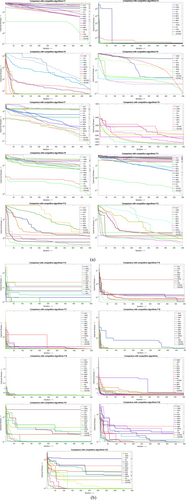
The comparative convergence curve shows that the IGOOSE algorithm outperforms many existing algorithms in terms of convergence speed and precision while maintaining strong competitiveness across a wide range of optimization problems. This rapid convergence is particularly evident when dealing with complex, high-dimensional optimization problems, where many other algorithms either stagnate or converge at a slower rate. The IGOOSE algorithm's robustness and effectiveness are evident when compared to existing algorithms such as HHO, GWO, and MPA. The IGOOSE algorithm is a superior choice for optimization tasks compared to other algorithms listed.
Table 3 focuses on a 10-dimensional, 50-dimensonal, 100-dimensonal search space, and the proposed IGOOSE algorithm consistently outperforms the GOOSE algorithm. For most functions, IGOOSE achieves lower average, best, worst, and median values, along with reduced standard deviation. For example in Table 3, in F1 and F2, IGOOSE achieves lower average error values (5.63E-05 and 0.015331, respectively) compared to GOOSE (3.6E-05 and 0.020684), indicating higher precision and robustness. Similarly, in functions like F3, F8, and F10, IGOOSE maintains a significant edge by delivering better best-case performance and smaller standard deviation, showcasing its stability and reliability in optimization tasks. Table 4 expands the comparison to a 30-dimensional (F1 to F13) and different-dimensional (F14 to F23) search space, where IGOOSE is compared against other state-of-the-art algorithms such as TLBO, WOA, GSA, WSO, GWO, MPA, TSA, and MVO. The results depict that IGOOSE consistently achieves better or comparable performance across various functions. While comparing with other algorithms, the proposed IGOOSE algorithm highlights its effectiveness in handling complex, multimodal functions. In total, the results clearly indicate that the IGOOSE algorithm not only outperforms its predecessor, GOOSE but also exhibits superior performance compared to a wide range of existing optimization algorithms, particularly in terms of accuracy, consistency, and stability across different dimensions and benchmark functions.
4 Optimal Engineering Structural Design Problems
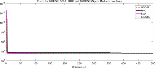
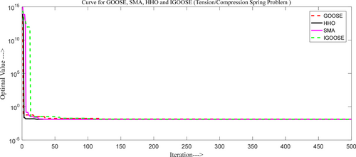
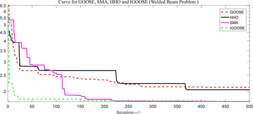
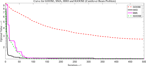
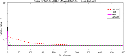
The structural engineering problems analyzed in this study include various real-world design optimization tasks such as minimizing weight and cost across different structural elements like the Three-Bar Truss, Speed Reducer, Pressure Vessel, and Welded Beam. Each problem is associated with specific objectives, constraints, and variables, as detailed in Table 8, which also presents the corresponding optimal structure figures, comparative convergence curves, and analysis tables. For instance, the Three-Bar Truss and Speed Reducer designs focus on weight minimization, while the pressure vessel and Welded Beam aim to minimize cost. The proposed IGOOSE algorithm's performance in solving these problems is summarized in Table 9, which reports simulation outcomes across multiple metrics, including average, best, worst, and median values. The algorithm consistently demonstrates superior performance, particularly in achieving lower fitness values, as observed in the Three-Bar Truss and Speed Reducer problems. Additionally, statistical significance is confirmed through Wilcoxon p values and T-test results, validating the algorithm's effectiveness. The convergence times also indicate the efficiency of IGOOSE in handling complex optimization tasks across different structural designs. The proposed IGOOSE algorithm's convergence for each optimal design structure was compared with the recent novel classical GOOSE algorithm, SMA, and HHO. From the comparative convergence analysis, the proposed IGOOSE algorithm demonstrates the fastest convergence and is competitive with other recent novel algorithms.
4.1 Three-Bar Truss Optimal Structure
Figure 5 presents the structure of three-bar truss problem.
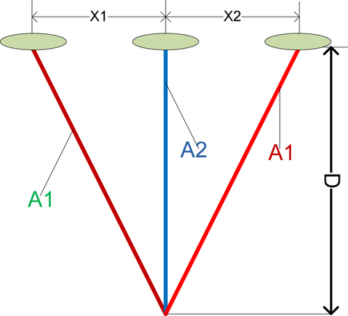
Here, l = 100 cm, p = 2KN/, = 2 KN/.
In Table 10, the proposed IGOOSE algorithm outperforms other optimizers in the three-bar truss optimization problem, achieving values of (x1, 0.784789) and (x2, 0.44224) with the lowest fitness score of 263.89598.
This fitness score is on par with GOOSE (263.89599) and slightly better than others like ZOA (263.896124) and MFO (263.8959797). Compared to methods like AOA (263.9154) and Ray and Sain (264.3217937), IGOOSE offers a more precise and optimized solution, demonstrating its effectiveness in this structural optimization task. Figure 6 presents a comparative convergence curve for the three-bar truss problem.

4.2 Speed Reducer Problem Optimal Structure
Figure 7 presents the structure of speed reducer problem. From Table 11, the proposed IGOOSE algorithm excels in the Speed Reducer optimization problem, achieving values of (x1, 3.523453), (x2, 0.7), (x3, 18.85562), (x4, 7.3), (x5, 7.830635), (x6, 3.423689), and (x7, 5.490621) with the lowest fitness score of 2998.419. Table 11 presents the proposed IGOOSE algorithm statistical comparative analysis for speed reducer optimal problem.
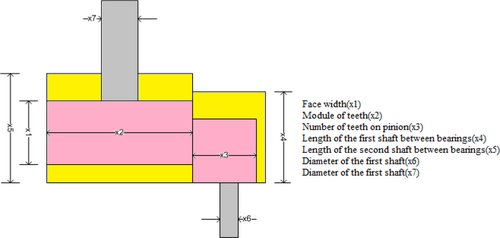
Here, .
This fitness score outperforms GOOSE (3002.622) and other methods like AO (3007.7328), SCA (3030.563), and GA (3067.561). IGOOSE's superior fitness value demonstrates its effectiveness in producing more optimal solutions, particularly in balancing the various parameters compared to other optimization techniques. Figure 8 presents the comparative convergence curve for the speed reducer problem.
4.3 Pressure Vessel Problem Optimal Structure
Figure 9 presents the structure of pressure vessel problem.

The proposed IGOOSE algorithm statistical comparative analysis for pressure vessel optimal problem is presented in Table 12. Figure 10 shows the comparative convergence curve for the pressure vessel problem.
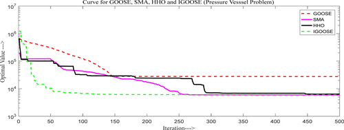
From Table 12, the proposed IGOOSE algorithm demonstrates superior performance in the pressure vessel optimization problem, achieving values of (Ts, 3.434804), (Th, 1.716901), (R, 177.8315), and (L, 23.82566) with the lowest fitness score of 5908.504. This fitness score is significantly better than GOOSE (6187.455) and other methods like WOA (6059.741) and GWO (6051.5639). Compared to algorithms like AOA and AO, IGOOSE excels in achieving an optimal balance across all parameters, making it highly effective in generating optimized solutions.
4.4 Tension/Compression Spring Problem Optimal Structure
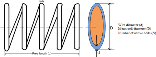
Figure 11 shows the structure of tension/compression spring problem. Table 13 presents the proposed IGOOSE algorithm achieves superior performance for the pressure vessel optimal problem.
Variable ranges, .
From Table 13, the proposed IGOOSE algorithm demonstrates outstanding performance in optimizing the pressure vessel problem, achieving values of (d, 0.058022), (D, 0.413332), and (N, 11.54606) with a leading fitness score of 0.012697. This fitness score surpasses that of GOOSE (0.012709) and other methods like WOA (0.012838) and PSO (0.014429). It also competes closely with PO (0.0126720) and OBSCA (0.012625), highlighting IGOOSE's effectiveness in producing highly optimized solutions compared to other optimization techniques.
Figure 12 shows the comparative convergence curve for the tension/compression spring problem.
4.5 Welded Beam Problem Optimal Structure
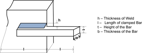
Figure 13 depicts the structure of welded beam problem. Table 14 presents the proposed IGOOSE algorithm statistical comparative analysis for welded beam optimal problem.
Variable range 0.1 2, 0.1 10, 0.1 10, 0.1 2.
From Table 14, the proposed IGOOSE algorithm excels in optimizing the Welded Beam problem, achieving the lowest values for (h, 0.63469), (l, 1.979674), (t, 3.773119), and (b, 1.239965), with a fitness score of 1.733172. This fitness score outperforms other methods like GOOSE (1.838048), SCA (1.77273347), and WOA (1.79061977), and significantly better than traditional methods such as GA, DAVID, and SIMPLEX, which have higher fitness values around 2.43–2.5307. This demonstrates IGOOSE's superior capability in generating optimized solutions for this problem. Figure 14 depicts the comparative convergence curve for the welded beam problem.
4.6 Belleville Spring Problem Optimal Structure
Figure 15 shows the structure of Belleville spring problem. From Table 15, the analysis of the Belleville Spring Optimal Problem shows that the IGOOSE algorithm outperforms other optimization methods. Figure 16 shows the comparative convergence curve for the Belle Ville Spring problem.


It achieves the lowest average fitness value (8.714061) and demonstrates greater consistency with a lower standard deviation (4.261281). Compared to alternatives like GOOSE and WOA, which have higher fitness values and variability, IGOOSE provides more reliable performance. Additionally, IGOOSE maintains near-optimal final objective values, surpassing other algorithms like ALO and ABC. Overall, IGOOSE proves to be the most effective and stable solution for optimizing the Belleville Spring problem.
4.7 Cantilever Beam Problem Optimal Structure
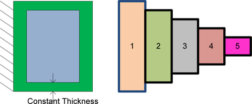
Figure 17 shows the structure of cantilever beam problem. From Table 16, the proposed IGOOSE algorithm shows superior performance in optimizing the Cantilever Beam problem, achieving the lowest (L1, 5.229071), (L2, 4.960867), (L3, 7.868921), (L4, 2.956664), and (L5, 5.699115) values with a competitive fitness score of 1.303286.
Variable ranges are, .
This fitness value matches closely with GOOSE (1.303279) and outperforms other optimizers like PKO, EOA, and SMA, which all have slightly higher fitness values around 1.33996. This highlights IGOOSE's efficiency in producing balanced and optimized solutions. Figure 18 shows the comparative convergence curve for the Cantilever beam problem.
4.8 I Beam Problem Optimal Structure
Figure 19 shows the structure of I beam problem. Table 17 presents the proposed IGOOSE algorithm statistical comparative analysis for I beam optimal problem.
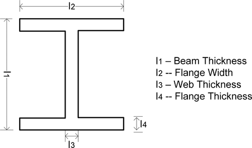
From Table 17, the proposed IGOOSE algorithm outperforms other optimizers in the I-Beam optimization problem, achieving the lowest (I1, 34.68268) and (I2, 71.13198) values, with a competitive (I3, 1.576975) and (I4, 4.993863) [94-98]. It matches the best fitness value (0.006626) alongside GOOSE and SMA, significantly better than ARMS, IARMS, SOS, and CS (0.0131). This indicates IGOOSE's superior efficiency in optimizing structural design, offering more balanced and precise solutions compared to other methods. Figure 20 shows the comparative convergence curve for the I beam problem.
5 Conclusion
The Random Walk-based Goose Search (IGOOSE) algorithm leverages the balance between exploration and exploitation by integrating random walk behavior with local search strategy. Extensive testing across 23 benchmark functions with varying dimensions (10, 30, 50, and 100) has demonstrated IGOOSE algorithm efficacy in different optimization search landscapes, with assessments based on solution quality, convergence speed, and robustness. Beyond theoretical benchmarks, IGOOSE algorithm has been successfully applied to eight distinct structural engineering designs, showcasing its versatility and effectiveness in practical structural engineering scenarios, including mechanical and civil engineering. The proposed IGOOSE algorithm has demonstrated superior performance compared to existing algorithms, including classical GOOSE. Across various benchmark functions, IGOOSE consistently outperforms GOOSE and other state-of-the-art search algorithms such as TLBO, WOA, GSA, WSO, GWO, MPA, TSA, and MVO. For instance, in a 10-dimensional search space, IGOOSE achieves lower average, best, worst, and median values, as well as reduced standard deviation, indicating higher precision and robustness. This trend continues across 30-dimensional and different-dimensional search spaces, where IGOOSE consistently delivers comparable or better performance, particularly in handling complex, hybrid, and multimodal functions. In structural engineering applications, IGOOSE has excelled in various optimization problems. In the three-bar truss problem, IGOOSE achieved the lowest fitness score of 263.89598, outperforming classical GOOSE and other methods like ZOA and MFO. In the Speed Reducer problem, IGOOSE outperformed classical GOOSE and other methods like AO, SCA, and GA with the lowest fitness score of 2998.4190. Similarly, in the pressure vessel problem, IGOOSE achieved a significantly better fitness score of 5908.5040 compared to classical GOOSE, WOA, and GWO. Also, in the Welded Beam problem, IGOOSE outperformed other methods, achieving the lowest fitness score of 1.733172, demonstrating superior capability in generating optimized solutions. Further, IGOOSE has shown its superior performance in optimizing the Belleville Spring problem, by achieving the lowest average fitness value and greater consistency with a lower standard deviation compared to alternatives like classical GOOSE and WOA. In the Cantilever Beam problem, IGOOSE achieved the lowest fitness score of 1.303286, matching closely with classical GOOSE and outperforming other optimizers like PKO, EOA, and SMA. Similarly, in the I-Beam problem, IGOOSE achieved the best fitness value of 0.006626, matching GOOSE and SMA, and significantly outperforming methods like ARMS, IARMS, SOS, and CS. In each case study of evaluation, the proposed IGOOSE algorithm proves to be a highly effective and stable solution across a wide range of optimal problems, consistently outperforming its predecessor, classical GOOSE, and other state-of-the-art algorithms. Its ability to achieve high accuracy, consistency, and stability across different-dimensional and benchmark functions makes it a valuable addition to the toolkit of optimization search practitioners. IGOOSE algorithm however provides the very competitive results when compared to tested algorithms but still the application of various strategies may further improve the performance of the algorithm. These strategies may be the hybridization with other algorithms, application of machine learning, and inclusion of a chaotic map in the proposed algorithm etc. The testing of the algorithm however to some extent guarantees its better performance bit still for complex related to mechanical and electrical engineering problems, the search space becomes complex and the algorithm may stuck at local minima which may provide hindrance to finding global solution to the problem.
Author Contributions
Sripathi Mounika: conceptualization, methodology, visualization. Himanshu Sharma: validation, methodology, investigation. Aradhala Bala Krishna: conceptualization, formal analysis, software, data curation. Krishan Arora: validation, software, formal analysis. Syed Immamul Ansarullah: writing – original draft, investigation, data curation, resources. Ayodeji Olalekan Salau: formal analysis, methodology, writing – review and editing, validation.
Acknowledgments
The authors have nothing to report.
Conflicts of Interest
The authors declare no conflicts of interest.
Open Research
Data Availability Statement
The data that support the findings of this study are available from the corresponding author upon reasonable request.


