State Identification of Charging Module Based on SN-EMD-SSEE and DBO-HKELM
Funding: This work was supported by Science and technology projects of State Grid Corporation of China, TSS2022-08.
ABSTRACT
Lithium-ion batteries are widely used in emergency back-up power supply with its superior performance, and they are usually used with a charging module. The charging module is usually composed of power electronic devices, but failures may occur in power electronic devicesdue to device aging and mechanical vibration in the complex environment; it will result in huge economic losses. However, the protection function of the charging module covers short fault, over-voltage fault, and over-current at system level rather than the open-circuit fault of MOSFETs and diodes at component level, which leads to hidden fire danger or accident risks. To address this issue, this paper improved a new state identification method of charging module based on signal normalization (SN) which is specially designed, empirical mode decomposition (EMD), sequence signal entropy extraction (SSEE), hybrid kernel extreme learning machine (HKELM), and dung beetle optimization (DBO). In basic work, 10 measurable variables and 23 fault states are determined by simulating open-circuit faults at MOSFETs and diodes. In data pre-processing, SN-EMD-SSEE is developed to extract state characteristics values for high adaptability to full working condition and high significance for easy identification. In modeling, DBO-HKELM identification model is constructed by improving ELM (Extreme Learning Machine) and optimizing parameters based on DBO 60 state characteristics values and 24 states including normal state, which are, respectively, used as the input and output of the identification model. In verification, the proposed state identification method based on SN-EMD-SSEE and DBO-HKELM is embedded into the control chip of charging module to obtain fault state code in real time. The experimental results show that the proposed state identification method is robust, and its identification accuracy is up to 94.7%.
1 Introduction
With the rapid development of power systems incorporating new energy sources in recent years, lithium-ion batteries have become increasingly popular as emergency backup power supplies for power stations. However, due to the crucial importance of charging safety, the charging module must possess a reliable stable control strategy [1]. Consequently, there is a pressing need to identify fault types and locations in a timely and accurate manner [1, 2]. The output characteristic of the converter is controlled by changing the duty cycle. Varying duty cycles cause small voltage and current fluctuations or a significant change, which results in reduced system stability and its equivalent parameter degradation, even the occurrence of open-circuit and short-circuit faults [2-5]. The fault-induced surge current can cause serious damage to other components. Power electronic switch devices are the weakest link in the reliability of charging modules, and the early diagnosis of their abnormal or fault can assist fault-tolerant operation or fault protection, which is crucial for the safety of battery charging [6-8]. The method of fault diagnosis mainly adopts an analytical model, data-driven technology, and a signal-processing method [9].
Using the method based on the analytical models, circuit operation states are simulated, and voltage or current is predicted, which are compared with their reference value [6, 10]. Then we can find out the abnormal state of the circuit operation. It usually uses the residual values of the phase currents obtained [7] to realize the diagnosis. Although the method can achieve faster fault diagnosis and accurate fault localization, the fault evolution mechanism requires the model with high accuracy, which leads to difficulty in modeling. Data-based modeling methods are usually built on the modeling framework under offline conditions. It usually uses expert systems [8, 9], support vector machines [11], neural networks [3], and other artificial intelligence algorithms to analyze and classify the fault signals that exhibit fault characteristics. Then it constructs the corresponding network model to carry out training and achieves scientific and accurate diagnosis. Signal processing decomposes and transforms the data according to the signal analysis strategy and extracts feature information from it [12-14]. Diagnostic methods can be divided into spectrum analysis method1 and wavelet transform method [15, 16]. Fault diagnosis and identification can be realized by comparing the change rule of feature information before and after the fault, and the diagnosis time is short, but for the complex system fault, the accuracy of this method will decrease.
- Based on the simulation and experiment environment, a fault simulation system of the charging module is established to study the change of input and output characteristics before and after a kind of fault occurs.
- To accurately identify charging module fault types and fault locations, charging module faults are meticulously categorized and encoded, with a total of 23 fault modes.
- According to the different characteristics of different faults, the fault feature vector is extracted from the input and output, the state feature extraction method SN-EMD-SSEE is proposed to improve adaptability and signification, and a generalized state identification model DBO-HKELM is developed, which greatly improves the accuracy and speed of fault diagnosis.
- The state identification method based on SN-EMD-SSEE and DBO-HKELM model has been proven to be accurate and robust through numerous fault simulation experiments.
2 Related Basic Work
2.1 Main Circuit and Its Measured Variables
Figure 1 shows the main circuit of charging module, including the front-stage circuit for rectifying and boosting and the secondary circuit for electrical isolation and current modulation. The front-stage circuit consists of six diode VDi (i = 1, 2, 3, 4, 5, 6) with a filter capacitor CVD in 3-Ph, two MOSFETs (S0 and ) with anti-parallel diodes (D0 and ) and coupling capacitors (C0 and ), a filter capacitor Cb, a diode Db, and an inductor Lb for continuous current in boost circuit. The secondary circuit consists of four MOSFETs (S1 and , S2 and ) with anti-parallel diodes (D1 and , D2 and ) and coupling capacitors (C1 and , C2 and ) in switching power supply, a resonant capacitance Cr, a resonant inductor Lr and an excitation inductor Lm in LLC converter, ideal transformer and two diodes (D3 and D4), and a filter capacitor C3 for 1-p full wave rectifier at its output side. uA, uB, and uC are input voltages. iA, iB, and iC are input currents. io is the operating current at the output side of module. vo is the output voltage, equal to the value of battery voltage. In addition, the operating temperature (T0 and , T1 and , T2 and ) of every MOSFET is monitored.

2.2 Simulation Model and Experimental Platform
To prove the validity and feasibility of the fault identification method proposed in this paper, both the simulation system and experimental platform of the charging module are built, as shown in Figure 2. The main device types used in the platform are as follows: Boost-PFC (Power Factor Correction) circuit inductor model th6-9021.3, size 940 MF, Diode Model C4D15120D, IGBT model IKW40N120H3, Negative Temperature Coefficient (NTC) thermistor CWF4B 103j3950. The simulation of the open circuit fault of diodes and switches at different positions is carried out. The input and output current and working temperature of the charging module are monitored by an oscilloscope.
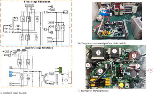
Figure 2c shows the top view of (b), where 1 to 6 are the transformer, resonant inductor, inductor of the pre-stage boost circuit, output filter capacitor, resonant capacitor, output filter capacitor, and main control chip.
To improve the robustness of the diagnostic method, the input voltage is set at intervals within ±15% (i.e., 187V˜264V) of its rated value (i.e., 220VAC), and the output voltage is set at intervals within ±10% (i.e., 198V˜286V) of its rated value (i.e., 220VDC), the simulation of the full operating condition is realized.
2.3 Fault Simulation
We consider the most common failures, which are open-circuit faults, short-circuit faults, and abnormal operating temperatures of MOSFETs or diodes in operation. For charging modules, short-circuit, over-current, and over-voltage faults are protected, but the deterioration and open-circuit faults of MOSFET or rectifier diodes are not in the full scope of protection functions. The simulation results of unprotected faults are shown in Figure 3.
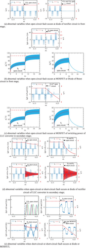
In order to study the characteristics of the electrical changes that occur when the fault occurs, the simulation software is used to simulate the electrical characteristics of the input current output current when the fault occurs at 0.2 s as shown in Figure 3. (a) The input and output currents of the electrical waveforms for the front-stage rectifier circuit diode when the open-circuit fault, occurs. We can see that a single open-circuit only corresponds to the phase missing half of the input, two open-circuit loss of all the input of the phase, the output in a short period of time with almost no change. (b) The figure shows the electrical waveforms and temperature simulation waveforms of the input and output currents when an open-circuit fault occurs in the diode or MOSFET of the preamplifier circuit. It can be seen that the input current slowly increases and the output current slowly decreases when an open-circuit fault occurs in the diode Db of the former circuit. When an open-circuit fault occurs in the power tube S0, there is no change in the input and output for a short period of time because the circuit uses two tubes running in parallel, but the temperature graph shows that the temperature of decreases and the parallel operation of the non-faulty tube S0 rises and stabilizes with a temperature change of about 10 s. (c) The figure shows the waveforms of the electrical and thermal characteristics of the back-stage circuit LLC during an open-circuit failure of the parallel MOSFET tubes in the bridge arms. When an open-circuit fault occurs in the parallel dual power tubes in either bridge arm, it can be seen that the input drops rapidly to 0 and the output drops rapidly to near the 0 value. When an open-circuit fault occurs in a single power tube S1 in any bridge arm, there is no effect on the input as well as the output for a short period of time because each bridge arm is running dual tubes in parallel, but the temperature graph shows that the temperature of S1 decreases and the parallel operation of the non-faulty tube rises and stabilizes with a temperature change of about 10 s. (d) The figure shows the electrical waveforms of the input and output currents of the rear output rectifier diode when an open-circuit and a short-circuit fault occurs. The electrical waveform of the input and output currents when D3 is open circuit, the peak value of the input current decreases slightly when D3 is open circuit and the output current decreases from 4 to 3, when D3 and D4 are open circuit at the same time, the input current attenuates to 0 within 0.05 s and the output current attenuates to 0 within 0.052 s, and the output current begins to gradually attenuate when D3 is short-circuited and the output current instantly becomes a sinusoidal waveform with a peak value of 2 from 4A to 2 when D3 and D4 are short-circuited. D3 and D4 short-circuit when the input current begins to gradually decay output current from DC 4A into the peak value from 4 to start decaying sine wave; (e) Figure for the part of the device occurs when the short-circuit failure of the input and output currents of the electrical waveforms, when the VD1, Db, or any of the MSOFET short-circuit, the input current suddenly increased for the original thousands of times and the output current output also shows a different degree of downward trend.
From Figure 3, it can be seen that we can extract fault characteristic parameters from the measured variables, iA, iB, iC, io, Ti, and .
3 Method Design
We proposed a new charging module state identification method based on SN, EMD, SSEE, ELM, and DBO, shown in Figure 4. Firstly, the data pre-processing link, SN-EMD-SSEE, is designed to reconstruct state characteristic values from measured current and temperature under all working condition with fault occurrence at given time point. Among them, SN is special made for 3-p input current, output current, and working temperature. Secondly, the state identification model DBO-HKELM is developed by using state characteristic values SN-EMD-SSEE as its input. It involves data set division, model selection and parameter optimization, model training, and model validation. Among them, we improved DBO and HKELM for high precision, and both RMSE and MARE are used for precision assessment. Finally, the state identification based on SN-EMD-SSEE and DBO-HKELM with the optimal parameters is embedded into the charging module for real-time real-time state monitoring.
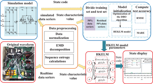
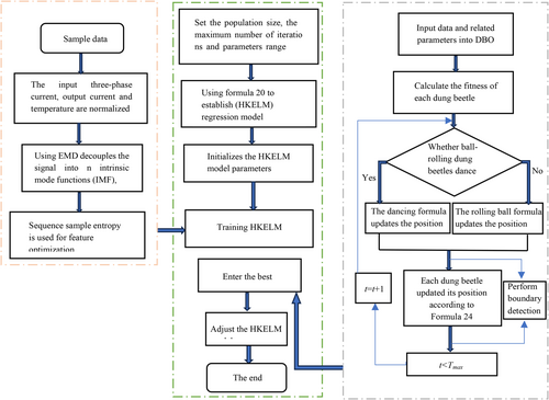
Firstly, the signal is normalized, and then the non-stationary data are smoothed by the EMD (empirical mode decomposition), so that the complex signal is decomposed into a finite IMF (intrinsic mode function) based on the given battery charge and discharge experimental data, the training set and test set are divided, and the input data of the original training set and test set are unified, that is, the input quantity is processed based on the maximum and minimum homogenization principle, and then the features were extracted by Sequence Sample Entropy Extraction. Secondly, introducing the DBO algorithm to optimize the HKELM model parameters, the DBO algorithm divides all mantises in the population into four distinct subpopulations, simulating the five behaviors of rolling ball, dancing, breeding, foraging, and stealing. The positions of the five mantis subpopulations are updated according to the formula iteratively until the number of iterations t reaches the maximum number of iterations Tmax and output the optimal solution of each parameter of the HKELM model to be optimized. So the regularization coefficient C, the mixed kernel parameters σ, m, n, and d, and the weight coefficient λ of the HKELM model were optimized by using dung beetle optimizer (DBO). Finally, the initial values of the optimal network parameters were obtained by the DBO algorithm, and the HKELM model was trained to obtain the global optimum. The feature signal is input into HKELM, and the overall optimization of the model performance is realized. The specific algorithm flowchart is shown in Figure 5.
3.1 Signal Normalization
- The normalized input current is defined as follows:
- The normalized output current is defined as follows:
- The normalized working is defined as follows:
3.2 Empirical Mode Decomposition
In Equation (4), x(t) is the original signal, ci(t) is the i-th IMF component, which contains the components of the original signal in different frequency bands and different time scales, and rn (t) is the trend component, which represents the average trend information of the original signal.
The IMF component should satisfy the following: (1) the sum of the extreme points should be equal to the number of points over zero or at most one difference; (2) the upper and lower envelopes are locally symmetric on the time axis.
- Determine all local extreme points of x(t) and connect the local value points with a cubic spline to form the upper envelope v1(t) and the lower envelope v2(t). The v1(t) and v2(t) are the upper and lower envelopes formed by connecting the local extreme points to the cubic spline, and compute the mean value m(t):
- Calculate h10(t):
- Calculate rn(t):
3.3 Sequence Sample Entropy Extraction
- N − m + 1 vector sequence with dimension m is extracted by ordinal number Xm(i), (i = 1, 2, …,N − m + 1). Calculate the distance between Xm(i) and Xm(j):
- Given r(r > 0), count the number of d [Xm(i), Xm(j)] less than r for each I, calculate its ratio to the total number of distances N-m, marked as :
- N − m vector sequences with m + 1 dimension Xm+1(i) are extracted by ordinal number, (i = 1,2, …, N − m). There are:
- The entropy of sequence sample EnSample(m,r) is calculated as:
The sample entropy is closely related to the sequence dimension M and the threshold R. Some studies suggest that m is usually set at 1 or 2, and R is usually set at 0.1–0.25 STD (the standard deviation from the original data). In this paper, m takes the value 2 and R takes 0.1 STD.
3.4 Hybrid Kernel Extreme Learning Machine
Considering the limitations of global and local cores, the traditional single-core function KLEM model is difficult to accommodate the nonlinear time-varying characteristics of the data samples such as voltage, current, and temperature in the battery dataset during random use. In order to further improve the prediction accuracy of KELM model, this paper combines the advantages of both global and local cores. The complex mixed core function is constructed by using RBF and Poly core functions, and the HKELM model is constructed by using the mixed core function to enhance the non-linear modeling ability. The xi represents the i th input sample. The yj represents the actual output of the ELM. The ωn and βm represent the random input weight between the ith hidden level node of the network and the input node and the output weight with the output node, respectively, bi represents the ith hidden layer offset, and g(x) is the activation function of the hidden layer. This method combines the advantages of ELM and multiple kernel functions, with a strong learning ability and generalization ability. The structure of HKELM neural network is shown in Figure 6.
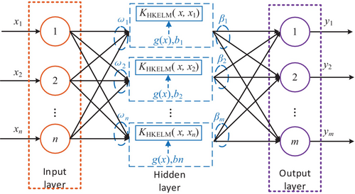
HKELM combines the advantages of kernel method and the ELM to achieve more efficient and accurate regression and classification tasks. HKELM not only inherits the fast training speed and generalization ability of ELM, but also improves the processing ability of the model to the complex data, thus realizing the overall optimization of the model performance.
3.5 Dung Beetle Optimizer
Dung Beetle Optimizer (DBO) [26, 27] is an optimization algorithm that simulates the behavior of Dung beetles in nature and is used to solve global optimization problems. In this paper, the DBO algorithm is introduced to optimize the regularization coefficient C, the mixed kernel parameter σ, m, n, and d, and the weight coefficient λ of the HKELM model with the root mean square error as the fitness function.
The DBO algorithm divides all dung beetles in the population into four different sub-populations and simulates five behaviors, namely, ball-rolling, dancing, reproduction, foraging, and stealing [15].
Finally, according to the Equations (8-11), by having different types of mantises perform their corresponding operations, the position and fitness of the subpopulation of dung beetle were updated continuously until the number of iterations t reached the maximum number of iterations Tmax, and the optimal solution of the parameters of the HKELM model to be optimized was the output.
4 The Results of the Experiment
4.1 State Encoding and Risk Description
According to the time-domain characteristics of these variables, we designed three kinds of risk levels G, Y, and R, whichcorrespond to no risk level, low risk level, and high risk level. The risk level R corresponds to the out-of-bounds failure; some variable exceeds its range, which is determined by the protection values or the limit value of the overload state. The risk level G is for no or slight deterioration of components and electrical contacts, corresponding to normal operating conditions; every variable changes in a certain range which is generally determined by rating value and coefficient of use of reduction. The Y level is between G and R, which is usually caused by progressive deterioration and is not to be ignored. We set the risk level threshold of state characteristic, shown in Table 1.
| Variable symbol | State characteristics | Threshold of risk level G | Threshold of risk level R |
|---|---|---|---|
| iK k = A, B, C | EnSampleIk k = A, B, C | ENIGY, the maximum of EnSampleIk from under 110% rating input current in normal state | ENIYR, the minimum of EnSample of from under 90% steady input current in unprotected fault state |
| io | EnSampleo | ENOGY, the maximum of EnSampleo from under 110% expected output current under initial state | ENOYR, the minimum of EnSampleo from under 90% output current in unprotected fault state |
|
Ti or k = 0, 1, 2 |
EnSampleTi or EnSampleTi* | ENTGY, the maximum of EnSampleo from under 10% unprotected operating temperature | ENTYR, the minimum of EnSampleo from under 90% unprotected operating temperature |
According to the risk level thresholds in Table 1, we can encode the fault modes corresponding to the state characteristics and location of the MOSFET or diode through the actual needs of the project, as shown in Table 2. The first column in the table is the fault number, the second column is the device type of the fault, the third column is the location of the fault, the fourth column is the description of the fault set by the simulated waveform, the fifth column is whether it is protected or not, and the sixth column is the risk level assigned according to the actual situation.
| Fault code | Fault mode | Fault location | Feature exception | Protection (yes or no) | Risk level |
|---|---|---|---|---|---|
| 0 | Normal | Nop | All EnSample no more than the threshold of risk level G | No | G |
| 1 | Open-circuit fault at single MOSFET | S0 | EnSampleT0* increase and EnSampleT0 decrease | No | R |
| 2 | Open-circuit fault at single MOSFET | EnSampleT0* decrease and EnSampleT0 increase | No | R | |
| 3 | Open-circuit fault at single MOSFET | S1 | EnSampleT1* increase and EnSampleT1 decrease | No | R |
| 4 | Open-circuit fault at single MOSFET | EnSampleT1* decrease and EnSampleT1 increase | No | R | |
| 5 | Open-circuit fault at single MOSFET | S2 | EnSampleT2* increase and EnSampleT2 decrease | No | R |
| 6 | Open-circuit fault at single MOSFET | EnSampleT2* decrease and EnSampleT2 increase | No | R | |
| 7 | Open-circuit fault at two mosfets | S0 and | EnSampleIk = 0 and EnSampleT0 and EnSampleT0* | No | R |
| 8 | Open-circuit fault at two mosfets | S1 and | EnSampleo decrease and EnSampleT1 and EnSampleT1* | No | R |
| 9 | Open-circuit fault at two mosfets | S2 and | EnSampleo decrease and EnSampleT2 and EnSampleT2* | No | R |
| 10 | Open-circuit fault at two mosfets | S1 and |
EnSampleT1*and EnSampleT2 increase EnSampleT2*and EnSampleT1 decrease |
No | R |
| 11 | Open-circuit fault at two mosfets | S1 and S2 |
EnSampleT1*and EnSampleT2* increase EnSampleT2and EnSampleT1 decrease |
No | R |
| 12 | Open-circuit fault at two mosfets | S2 and |
EnSampleT2*and EnSampleT1 increase EnSampleT2and EnSampleT1* decrease |
No | R |
| 13 | Open-circuit fault at two mosfets | S2 and S1 |
EnSampleT1*and EnSampleT2* increase EnSampleT2and EnSampleT1 decrease |
No | R |
| 14 | Open-circuit fault at single diode | Db | EnSampleIk increase and EnSampleo decrease | No | Y |
| 15 | Open-circuit fault at single diode | D3 or D4 | EnSampleIk and EnSampleo decrease in lower speed | No | R |
| 16 | Open-circuit fault at two diodes | D3 and D4 | EnSampleIk and EnSampleo decrease in certain speed | No | R |
| 17 | Short-circuit fault at single diode | D3 or D4 | EnSampleIk decrease and EnSampleo jump down firstly and then decrease with oscillation | No | R |
| 18 | Short-circuit fault at two diodes | D3 and D4 | EnSampleIk decrease and EnSampleo decrease with oscillation | No | R |
| 19 | Open-circuit fault at two diodes | VD1 or VD4 | A phase missing only IA → 0 | Yes | R |
| 20 | Open-circuit fault at two diodes | VD2 or VD5 | B phase missing only IB → 0 | Yes | R |
| 21 | Open-circuit fault at two diodes | VD3 or VD6 | C phase missing only IC → 0 | Yes | R |
| 22 | Short-circuit fault at single diode | VDi, Db, Si or | A sudden increase in the input current EnSampleIk > 5ENIYR | Yes | R |
| 23 | Parameter degeneration | Module | ENGY < any EnSample < ENYR | No | Y |
Based on risk level thresholds in the table, we can encode the fault modes corresponding to the state features and the position of MOSFET or diode, listed in Table 2.
4.2 State Characteristics Extraction
We take the SSE of IMFi (i = 1,2, …, 6) of 10 normalized state variables within 20 ms after fault occurrence as state characteristics values for all faults of concern. In the case of fault 16, the range of 60 state eigenvalues is shown in Table 3.
| State characteristics values range after fault occurrence within 20 ms | ||||||
|---|---|---|---|---|---|---|
| Variable | IMF1 | IMF2 | IMF3 | IMF4 | IMF5 | IMF6 |
| iA | 0.503343 → 0.278251 | 0.406562 → 0.429045 | 0.585029 → 0.579311 | 0.513439 → 0.525709 | 0.318318 → 0.169359 | 0.048013 → 0.052107 |
| iB | 0.548936 → 0.600039 | 0.576956 → 0.449973 | 0.559490 → 0.616845 | 0.405833 → 0.547249 | 0.056448 → 0.236907 | 0.022263 → 0.064352 |
| iC | 0.548893 → 0.594078 | 0.529115 → 0.576637 | 0.572790 → 0.629547 | 0.409059 → 0.552813 | 0.090641 → 0.202375 | 0.087626 → 0.087626 |
| io | 0.1000 → 0.0000 | 0.1000 → 0.0876 | 0.1000 → 0.0300 | 0.1000 → 0.0151 | 0.1000 → 0.0037 | 0.1000 → 0.0001 |
| T0 | 0.498761 → 0.496604 | 0.539895 → 0.54196 | 0.569124 → 0.569241 | 0.527450 → 0.527419 | 0.377150 → 0.377139 | 0.218492 → 0.219498 |
| 0.490144 → 0.490428 | 0.552130 → 0.551272 | 0.56542 → 0.56232 | 0.533825 → 0.538277 | 0.172541 → 0.171158 | 0.034832 → 0.034734 | |
| T1 | 0.468917 → 0.468916 | 0.606350 → 0.606349 | 0.569871 → 0.57889 | 0.416450 → 0.416417 | 0.260504 → 0.260506 | 0.02336 → 0.023355 |
| 0.490125 → 0.490428 | 0.551278 → 0.551272 | 0.56312 → 0.56232 | 0.538276 → 0.538277 | 0.171157 → 0.171158 | 0.034751 → 0.034734 | |
| T2 | 0.515486 → 0.515486 | 0.608657 → 0.608656 | 0.503246 → 0.502345 | 0.398549 → 0.399573 | 0.108143 → 0.108142 | 0.033089 → 0.033089 |
| 0.403019 → 0.403045 | 0.318797 → 0.328797 | 0.462913 → 0.462911 | 0.349429 → 0.349436 | 0.129684 → 0.129684 | 0.023672 → 0.023670 | |
From Table 3, we can see that when a fault occurs after the EMD algorithm run processing results from the normal value in front of the arrow to the value behind the arrow, which can be used as a basis for determining whether the fault occurs and its location.
4.3 Identification Results
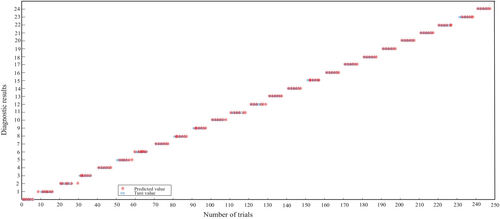
Some unprotected faults are simulated and identified using the identification method proposed in this paper under full working conditions on the experimental platform. Partial fault identification results are shown in Figure 7 and the fault statistics, the statistical results of identification accuracy are shown in Figure 8.
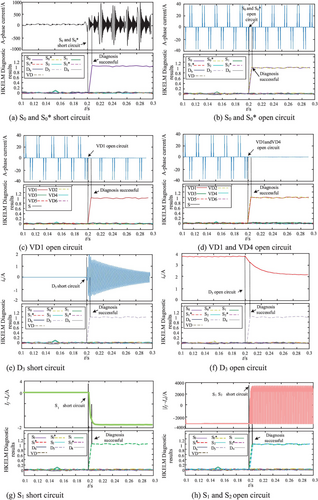
As shown in Figure 7a, the upper part of the figure is the decomposition waveform with obvious characteristics after data preprocessing and EMD decomposition, and the lower part is all the fault curves recognized by the model. When the fault occurs in 0.2 s, the upper part of the waveform undergoes a serious aberration after the model diagnosis of the fault recognition outputs the corresponding fault curves of the lower half. At this time, the corresponding fault curves rise rapidly from the vicinity of the value of 0 to the value of 1 neighborhood, representing the success of fault recognition. In Figure 7b, when the fault occurs, the upper part of the processing waveform cannot be connected and reversed, and the corresponding fault curve rises rapidly from near 0 to 1 neighborhood and represents the success of the fault identification; in Figure 7c, when a fault occurs, part of the upper half of the processing waveform is lost, the corresponding lower part of the fault curve of the diagnostic output of the fault identification model rises rapidly from the vicinity of 0 to the neighborhood of 1, representing the success of fault identification; in graph (d), when a fault occurs, in the upper part of the processing waveform, all the waveforms are lost, and the corresponding lower part of the fault curve rises rapidly from 0 to 1 neighborhood, which represents the success of fault identification; in Figure 7e, when the fault occurs, the upper part of the processing waveform part of the phenomenon of violent oscillation with positive and negative, the corresponding lower part of the fault curve of the diagnostic output of the fault identification model rises rapidly from the vicinity of 0 to the neighborhood of 1, representing the success of fault identification; in graph (f), when a fault occurs, the upper part of the processing waveform part slowly decays away from the normal value, and the fault identification model diagnosis output corresponding to the lower part of the fault curve rises rapidly from near 0 to 1 neighborhood, represents the success of the fault identification; in Figure 7g, when the fault occurs, the upper part of the processing waveform part appears to decline rapidly, the corresponding lower part of the fault curve of the diagnostic output of the fault identification model rises rapidly from the vicinity of 0 to the neighborhood of 1, representing the success of fault identification; in Figure 7h, when a fault occurs, in the upper part of the processing waveform, the amplitude on the side that deviates from the time axis rises rapidly and a severe oscillation occurs, the corresponding lower part of the fault curve rises rapidly from 0 to 1 neighborhood, which represents the success of fault identification.
Figure 8 shows the accuracy of using the DBO-HKELM fault diagnosis model, with the samples of faults used on the horizontal axis and the corresponding fault codes on the vertical axis, one fault code for each fault type and 10 samples for each fault type. The test was conducted 10 times for each fault type and the number of results was recorded as shown in Figure 8, so that the fault code corresponding to each fault type could be accurately diagnosed. Finally, based on SN-EMD-SSEE and DBO-HKELM, different faults can be accurately identified and localized with an accuracy of 97.6% and good robustness.
From Figures 7 and 8, it can be seen that the proposed state identification based on SN-EMD-SSEE and DBO-HKELM can provide accurate judgment and location of different faults with good robustness. Fault identification accuracy for MOSFETs or diodes is about 97.6% when additionally considering communication faults, sensor faults, and others.
4.4 Comparison of Fault Identification Methods
To prove the accuracy and validity of the proposed SN-EMD-SSEE and DBO-HKELM model, we select two fault feature extraction methods and four fault identification methods for comparison.
The diagnosis results of fault feature extraction using the original wavelet packet algorithm and Sequence Sample Entropy Extraction are shown in Table 4. It can be seen from the Table 4 that the fault feature extracted by the improved wavelet packet algorithm is more representative and the diagnosis result is better. Table 5 shows diagnostic results with other superior methods, namely ELM, GWO-ELM, DBO-KELM, and DBO-HKELM. It can be seen from Table 5 that the training accuracy and test accuracy of the proposed method are higher than those of the other three methods.
| Feature extraction | Training accuracy (%) | Test accuracy (%) |
|---|---|---|
| Original wavelet packet | 91.16 | 89.52 |
| Sequence Sample Entropy Extraction | 97.78 | 98.36 |
| Method | Training accuracy (%) | Test accuracy (%) |
|---|---|---|
| ELM | 96.20 | 92.30 |
| GWO-ELM | 97.06 | 97.20 |
| DBO-KELM | 97.50 | 97.05 |
| DBO-HKELM | 98.21 | 97.6 |
5 Conclusion
In order to meet the requirements of real-time monitoring of lithium-ion battery charging in case of open-circuit failure of charging modules MOSFET and diode, a state recognition method based on SN-EMD-SSEE and DBO-HKELM is proposed in this paper.
Three-phase AC input current, DC output current, and MOSFET operating temperature of the charging module are measured, and the normalization methods are designed, respectively. Furthermore, a data pre-processing method based on SN-EMD-SSEE is proposed to obtain the state characteristic parameters needed for identification. And the adaptability of the identification method to module power supply and load is improved.
DBO-HKELM model with good robustness and strong generalization ability is constructed based on ELM. Sixty state characteristic parameters with important fault information are extracted as input of the DBO-HKELM model. Twenty-five fault states are determined by fault simulation under full operating conditions and used as the output of DBO-HKELM model. Based on the training and testing of a large number of fault simulation data, the optimal parameters of the DBO-HKELM model are determined. The experimental results show that the identification method has good adaptability, robustness, and high accuracy of source load.
However, it is unable to locate the faults accurately and quickly by 100%, and it cannot be completely intelligent. It is expected that further improvement on the model can speed up the diagnosis time and diagnosis accuracy. Due to the large amount of data classification and summarization, the algorithm program does not run quickly, so in the future, we can further find more convenient and more representative forms of failure to speed up the overall running time.
Nomenclature
-
- C1 and , C2 and
-
- coupling capacitors for four MOSFETs in the secondary circuit
-
- Cr
-
- resonant capacitance in LLC converter
-
- CVD
-
- a filter capacitor for front-stage circuits
-
- D1 and , D2 and
-
- anti-parallel diodes for four MOSFETs in the secondary circuit
-
- D3 and D4
-
- 1-Ph full-wave rectifier diode at output
-
- Db
-
- diodes for PFC circuits with front-stage LLCs
-
- DBO
-
- Dung Beetle optimization
-
- ELM
-
- extreme learning machine
-
- EMD
-
- empirical mode decomposition
-
- HKELM
-
- hybrid kernel extreme learning machine
-
- Lr
-
- resonant inductor in LLC converter
-
- Lm
-
- excitation inductor in LLC converter
-
- LLC
-
- LLC converter
-
- io
-
- output currents of llc converter
-
- iA, iB, and iC
-
- input currents of llc converter
-
- NTC
-
- temperature coefficient thermistor
-
- PFC
-
- power factor correction circuit
-
- S0,
-
- two MOSFETs for front-stage circuits
-
- S1 and , S2 and
-
- four MOSFETs for secondary-stage circuits
-
- SN
-
- signal normalization
-
- SSEE
-
- sequence signal entropy extraction
-
- vo
-
- output voltage of LLC converter
-
- VDi
-
- rectifier diode voltage for front-stage circuits
-
- T0 and , T1 and , T2 and
-
- the operating temperature of every MOSFET
Author Contributions
Bingyu Li: conceptualization, investigation, visualization, validation, methodology, formal analysis, writing – original draft, writing – review and editing, data curation. Xianhai Pang: investigation, validation, formal analysis, writing – original draft. Xuhao Du: investigation, validation, visualization, writing – original draft, formal analysis. Ziwen Cai: investigation, validation, writing – review and editing, formal analysis.
Conflicts of Interest
The authors declare no conflicts of interest.
Open Research
Data Availability Statement
Data sharing not applicable to this article as no datasets were generated or analysed during the current study.


