Selection of Optimized Diagnostic Approach for Cardiovascular Diseases Leveraging Dynamic Linguistic Intuitionistic Fuzzy Decision-Making Technique
ABSTRACT
Fuzzy mathematical operations play an important role in the field of decision-making. Decision-making tools are being used in every field of life. Fuzzy operators are the building blocks for making a decision in the realm of uncertain information. The information is often in qualitative form which needs a qualitative approach for decision-making rather than a quantitative one. The linguistic term sets are the mathematical tools to collect the qualitative data from experts of the fields and the conversion of linguistic data in the form linguistic intuitionistic fuzzy data is the more efficient and reliable for the process of decision making. The fuzzy aggregation operators are the best tools for the aggregation of uncertain and vague data. This work addresses a real-world decision-making problem of choosing the best diagnostic approach for the diagnosis of cardiovascular diseases by introducing a novel decision-making technique with fuzzy aggregation operators in the domain of linguistic intuitionistic fuzzy (LIF) sets. Two new operators are used in this method: the Dynamic Linguistic Intuitionistic Fuzzy Dombi Weighted Averaging (DLIFDWA) operator and the Dynamic Linguistic Intuitionistic Fuzzy Dombi Weighted Geometric (DLIFDWG) operator. This work aims to identify an optimal technique for diagnosing cardiovascular illness using Dombi operations in the Linguistic Intuitionistic Fuzzy environment. The Dombi Operations are highly versatile and successful in addressing vagueness and uncertainty, making them crucial in our methodology. To demonstrate the effectiveness of the offered strategies, we have implemented the recommended operators for the selection of optimized diagnostic approach for cardiovascular diseases. This showcases the significance of these strategies in facilitating decision-making. Ultimately, we perform a thorough analysis to showcase the reliability and uniformity of the produced procedures, comparing the provided operators with various current counterparts.
Abbreviations
-
- CVD
-
- Cardiovascular Disease
-
- DLIFDWA
-
- Dynamic Linguistic Intuitionistic Fuzzy Dombi weighted Averaging
-
- DLIFDWG
-
- Dynamic Linguistic Intuitionistic Fuzzy Dombi weighted Geometric
-
- FS
-
- Fuzzy Set
-
- IFS
-
- Intuitionistic Fuzz Set
-
- IHME
-
- Institute for Health Metrics and Evaluation
-
- LIFDWA
-
- Linguistic Intuitionistic Fuzzy Dombi weighted Averaging
-
- LIFDWG
-
- Linguistic Intuitionistic Fuzzy Dombi weighted Geometric
-
- LIFN
-
- Linguistic Intuitionistic Fuzzy Number
-
- LIFS
-
- Linguistic Intuitionistic Fuzzy Set
-
- MADM
-
- Multiple Attribute Decision-making
-
- MAGDM
-
- Multiple Attribute Group Decision-Making
-
- MD
-
- Membership Degree
-
- NMD
-
- Non-membership Degree
-
- WHO
-
- World Health Organization
1 Introduction
The deployment of algorithmic decision-making systems has greatly improved the handling of large healthcare datasets, especially in the production of forecasts and diagnoses [1, 2]. Computer science, healthcare diagnostics, company management, and product selection in dynamic markets are just a few of the many fields that rely on strategic decision-making processes. Decision-making strategies cover many other fields like wine-making industry [3] and trajectory prediction of intelligent connected vehicles [4]. Within the framework of Multiple Attribute Decision Making (MADM), each attribute is assigned specific weights that have a distinct and significant impact on the decision-making process [5, 6]. The practical challenges of decision-making involve uncertainties and complexities that can be effectively addressed by using fuzzy sets (FS). Evaluation of ambiguous and uncertain data has demonstrated that it benefits from the application of Zadeh's idea of FS [7]. The membership degrees that lie inside the range [0, 1] are the main focus of the dynamical framework of a FS. Existing literature [8-10] acknowledges the difficulty in gathering attributes and minimizing the difference between them, which results in a stronger reliance on fuzzy environment. The scope of FS has grown over time, ignoring the issue of non-membership in favor of its original concentration on degrees of membership. In response, degrees of non-membership were introduced by Atanassov [11] in the context of intuitionistic fuzzy sets (IFS). In the mathematical expression, the degree of membership is represented as , and the degree of non-membership is represented as , with . Researchers have developed a variety of IFS-based solutions in a variety of domains to handle the difficulty of aggregating and measuring the distance between many characteristics. For example in the domain of IFS, Liu et al. [12] proposed a hybrid technique, Thao [13] looked into entropies and divergence measures while taking Archimedean norms into account, Gohain et al. [14] looked at the distance and similarity metrics, and Garg, Rani [15] identified and studied similarity measures. For further developments in the field of IFSs, the reader is recommended to read references [16-24]. Real-world decision-making problems often involve complex and ambiguous information. This makes it challenging to simulate these problems using fuzzy sets (FS) and intuitionistic fuzzy sets (IFS), as these sets can only express information in quantitative terms. In order to address these types of issues within the fuzzy field, Huiminn Zhang [25] proposed the notion of linguistic-IFS, which focuses on handling information in the qualitative domain. The field of linguistic intuitionistic fuzzy sets provides academics with the opportunity to address complex decision-making scenarios. Several researches have been undertaken in this field that demonstrate the efficacy of this approach. As an illustration, Yager [26] examined the ordinal LIFS method for assessing mobile apps. Rishu Arora and Harish Garg [27] explored the prioritized LIF aggregation operators and discussed their fundamental characteristics. Harish Garg and Kamal Kumar [28] devised power aggregation operators through set pair analysis within the domain of linguistic intuitionistic fuzzy sets, the challenge of combining several attributes and determining the optimal option based on these attributes is a challenging endeavor that captivates academics. A multitude of studies have been carried out to address the intricate issues related to decision-making [29-34].
1.1 Novelty, Goals, and Key Results of the Work
- In the domain of multi-attribute decision-making problems, two new dynamic operators have been created for aggregating fuzzy dynamic data that is Linguistic Intuitionistic fuzzy: the DLIFDWA operator and the DLIFDWG operator.
- The article offers a thorough and reliable explanation to accurately define the essential properties of operators, such as their monotonicity, idempotency, and boundedness which shows that these operators are capable of aggregating the dynamic natured data.
- The aforementioned operators play an important role in formulating a rational approach for the management of the outcomes of Multiple Attribute Decision Making (MADM) in the Linguistic intuitionistic fuzzy environment.
- The inclusion of generic parameter in the Dombi operations and also in the proposed operators makes them versatile in nature. It provides number of ways to handle uncertainty and vagueness. This nature of the operators make them best match for the real-world scenarios.
- The applicability of the proposed operators in real-world scenarios is demonstrated by applying them to a MADM problem, which entails identifying the most effective strategy for diagnosing cardiovascular sickness. The purpose of this real-world application is to evaluate the effectiveness of the suggested operators in improving decision-making processes.
- A comparative analysis of multiple prior studies substantiates the durability and effectiveness of the suggested methodology in real-world scenarios and shows the connection of the study with practical world.
Section 2 of this article contains a comprehensive analysis of essential definitions, which will be presented in the succeeding sections of this article. Section 3 provides an illustration of the dynamic operations that are carried out on LIFSs as well as the fundamental concepts that govern these operations. The dynamic aggregation operators in the framework of dynamic linguistic intuitionistic fuzzy data are researched and described in detail in the fourth section of this paper. A technique for making decisions that addresses concerns associated with a dynamic framework is detailed in Section 5. The operators that were recently devised are employed in Section 6 to determine the optimal approach for diagnosing cardiovascular disease. Furthermore, we provide a comparative analysis with the objective of elucidating the viability and efficacy of this distinctive approach in relation to traditional methodologies. In the conclusion, the study furnished a brief overview of the principal findings, accompanied by a few provisional suggestions.
2 Significant Definitions
Generally, the linguistic term set established above is proposed to a continuous linguistic term set by Xu [40] in order to reduce the loss of facts. Here, its justification is left out.
Definition 2.1.[11] In the discourse universe , the intuitionistic fuzzy set is represented by the set where, and represents the MD and NMD for each in the set , as well as and As for any , the indeterminacy or hesitation index in the set is . Xu and Yager [41] defined an intuitionistic fuzzy number (IFN) as the pair for a given if A is an intuitionistic fuzzy set.
Definition 2.2.[25] Given a continuous linguistic term set and , the linguistic intuitionistic fuzzy number (LIFN) is defined as the order pair , if .
Clarification. is also a LIFN, where and .
is used throughout this work to simply symbolize a set of all LIFNs.
Definition 2.3.[25] The following are the fundamental operating principles of the linguistic intuitionistic fuzzy numbers, assuming that , .
Definition 2.4.[25] If we assume that , then:
Show the scoring function and accuracy function of respectively.
Definition 2.5.[25] Let , then
- ( is smaller than ) if ,
- If , then
- ( is smaller than ) if
- ( and have the same information) if
3 LIFNs: Dynamic Operations
Informational aggregation is a key and major area of study in the field of information fusion. The combination of complicated intuitionistic fuzzy information using time-independent arguments is restricted to the procedures LIFWA and LIFWG. When taking into consideration the temporal component, it is essential to keep in mind that linguistic intuitionistic fuzzy data might be obtained at a variety of different moments in time. In situations like this, it is of the utmost importance to make certain that the aggregation operators and the weights that correspond to them are not maintained at a constant value. Therefore, we will initially establish the theoretical foundation of a Dynamic Linguistic intuitionistic fuzzy parameter in the subsequent sections, drawing from the work of [42].
3.1 Dynamic LIFNs' Operational Laws
We define the basic principles of a linguistic intuitionistic fuzzy dynamic variable and introduce the idea in this subsection.
Definition 3.1.1.We introduce a novel concept in mathematical language: a “dynamic linguistic intuitionistic fuzzy variable,” where represents a temporal variable. This variable is defined by the following constituents:
such that
These parameters also need to follow the restriction . More broadly, given a series of time occurrences, , then represent unique LIFNs, each corresponding to a particular time period. In the context of LIFNs, we define in Definitions 3.1.2 and 3.1.3 the basic ideas guiding their interactions.
Definition 3.1.2.Let and are two LIFNs at time periods and . Then, following are the fundamental operational laws which govern how they interact:
- if and
- if and only if and
Definition 3.1.3.The generic operations two LIFNs, and , together with a positive real scalar factor , can be expressed as follows:
4 Dynamic LIFNs' Dombi Operations
Definition 4.1.[43] Given any two real numbers and . The Dombi triangular-norm and triangular-conorm that result from are provided below:
Definition 4.2.The norms and co-norms are the operations that are used to combine the fuzzy membership and non-membership in a particular binary operation of fuzzy numbers. The versatility of the Dombi norm and co-norm encourages us to define these operations on the LIFNs. These operations are defined as follows:
Definition 4.3.The averaging operators are the best tools for aggregating a collection of data in the scenarios where the totality is based on summation. The averaging operators are monotonic, idempotent and bounded, these properties make them best choice for the aggregation of data concerned. The conversion of averaging operators in the realm of dynamic LIFS is defined as concerning various time periods , let be a set of n LIFNs, and let be the weight vector. The averaging operator for dynamic Linguistic Intuitionistic Fuzzy numbers is
Theorem 4.1.Let with be the associated weight vector to a collection of distinct LIFNs of LIFNs perceived at distinctive time periods , ranges from to and for a Dombi parameter . We have,
Proof: Now, based on the principle of induction.
Consequently, for , the result is valid.
Therefore, Theorem 4.1 is valid for .
As a result, this outcome holds true for any value of the positive integer .
Theorem 4.2.Let with be the associated weight vector to a collection of distinct LIFNs of LIFNs perceived at distinctive time periods , ranges from to and for a Dombi parameter . The operator has the subsequent characteristics:
-
If all LIFNs recorded in different time spans ( ranges from to ) are equal, that is , then
-
Let be another collection of LIFNs taken at distinct time periods ( ranges from to ) and if and for any , then
-
If , for any , then
- Since and for any .
Definition 4.4.The geometric operators deal with the aggregation of the data whose totality is based on the product of the collected data. The geometric operators in a dynamic linguistic intuitionistic environment are defined as consider be a collection of LIFNs taken at distinct time periods (ranges from to ) and is the affiliated weight vector. Then, the geometric operator for dynamic linguistic intuitionistic fuzzy numbers is defined as:
Theorem 4.3.For a collection of LIFNs at distinct time intervals and be the affiliated weight vector such that where, and Dombi parameter . Then, the clumped value of these LIFNs by the DLIFDWG operator is,
Proof: Now, based on the principle of induction.
Consequently, for , the result is valid.
Therefore, Theorem 4.3 is valid for .
As a result, this outcome holds true for any value of the positive integer .
Theorem 4.4.Let with be the associated weight vector to a collection of distinct LIFNs perceived at distinctive time periods , ranges from to and for a Dombi parameter . The operator has the subsequent characteristics:
-
If all the LIFNs taken at distinct time periods ( ranges from to ) are equal, that is , then
-
Let be another collection of LIFNs taken at distinct time periods ( ranges from to ) and if and for any , then
- The monotonicity property of operator ensures that it is bounded. That is,
5 Execution of and Operators in Decision-Making Strategy
Due to technological advancements over time, it is essential to replace traditional technologies in healthcare settings with more advanced alternatives. The implementation of any technology requires a thorough assessment concerning timeframes. The assessment of time-dependent approaches necessitates aggregation operators with a dynamic nature. The suggested operators are adaptable and capable of addressing time-sensitive information. These operators align effectively with real-world applications. We will provide a novel Multiple Attribute Group Decision Making (MAGDM) method based on the application of the DLIFDWG and DLIFDWA operators in the next section. An inclusive description is presented in the following:
Let represents the set of all attributes, and let represents all alternatives that are evaluated at time spans . Moreover, a weight vector is connected with each of the discrete time period designated as where , and . As the evaluation value of the alternative we utilize LIFN in accordance with the attribute taken at a discrete time period and . The following is a description of the suggested model.
5.1 Algorithm Incorporated With DLIFDWA
Step 1. Create LIF decision matrices to represent matrices at different time spans .
Step 3. Using the operator, aggregate to obtain the overall collective evaluation value of the alternative .
Step 4. Determine the scoring value of the evaluation value of alternatives . Sort down the alternate choices and select the best one based on the scores.
5.2 Algorithm Incorporated With DLIFDWG
Step 1. Construct the LIF decision matrices that are the matrices at different time periods .
Step 3. Aggregate to obtain the collective overall evaluation value of the alternative using LIFDWG operator.
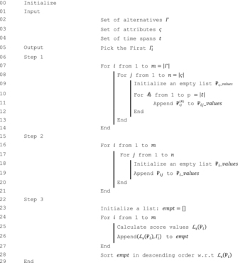
Step 4. Calculate the score of the evaluation value of alternatives . Based on the scores, rank the alternatives and pick the best one (Figure 1 and Algorithm 1).

ALGORITHM 1. Representation of the Proposed Dynamic MADM.
6 Application of Proposed Operators in MADM Problem
In the following section, we provide a numerical example to further clarify the previously described technique. Next, we contrast this example's results with those of previous studies.
6.1 Case Study
A wide variety of long-term illnesses that harm the circulatory system are collectively known as cardiovascular diseases (CVDs). A significant proportion of the American population displays frighteningly high levels of saturated fat, a condition that can present in several ways. Individuals suffering from this disease may opt to modify their lifestyle or see healthcare professionals and adhere to prescribed medication in order to manage the condition. Early detection of this disease enables a more positive treatment outcome. Cardiovascular disease is the leading cause of death globally and in the United States. Each year, an astonishing 655,000 people in the United States die from heart disease. Cardiovascular disease affects around 50% of the overall population in the United States. It impacts individuals of both sexes. Statistically, the mortality rate for women due to this particular disease is one in three. These phenomena impacts individuals of diverse age groups, ethnicities, and socioeconomic statuses. The main behavioral risk factors linked to cardiovascular disease (CVD) and stroke include smoking tobacco, excessive alcohol use, consumption of an unhealthy diet, and insufficient physical exercise. Adults exhibiting behavioral risk factors may experience elevated blood glucose levels, increased level of cholesterol, elevated serum lipids, and overweight or obesity. These intermediate risk factors are significant indicators of a higher probability of experiencing negative cardiovascular events, such as cardiac arrhythmia, hemorrhage, related complications, and myocardial infarction. It is justifiable to investigate and assess these risk variables in primary care settings. To mitigate the prevalence of cardiovascular disease, individuals and society at large can adopt several measures. These include abstaining from smoking, decreasing sodium consumption, including a higher proportion of fruits and vegetables into daily dietary habits, engaging in regular exercise, and consuming alcohol in moderation. People's healthy habits must be encouraged and maintained by health policies that make healthy options more inexpensive and accessible. It is also important to understand that the etiology of cardiovascular diseases is impacted by a variety of factors. Population aging, urbanization, and globalization are the three most important drivers of social, economic, and cultural development. Additional risk factors include genetic susceptibility, emotional strain, and socioeconomic hardship. The risks of cardiovascular events such as heart attacks and strokes are reducible by the utilization of clinical interventions targeting hypertension, diabetes, and increased serum lipid profiles. Cardiovascular disease caused of deaths in Pakistan as per stats of the World Health Organization (WHO). These stats show the dominance of the growth of this disease in Pakistan together with health risks like hypertension, hypercholesterolemia and high blood sugar. Cardiovascular disease and these health risks can be reduced by the adjustment of the lifestyle.
Gender, age and health history in the family are those risk factors for cardiovascular illness that cannot be modified. In general, men are more susceptible than women to suffer from cardiovascular disease, and this risk rises with age. An individual's risk of acquiring CVD is increased if there is a family history of the illness.
- Lifestyle decisions: The decision regarding a healthful lifestyle plays an important role in the promotion of the cardiovascular health and reducing the risks of the disease. A healthy lifestyle may be included discontinuation of the smoking habit and maintenance of an appropriate weight by adopting a balanced diet plan and frequent exercises.
- Pharmaceutical therapies: These approaches based on the maintenance of the proper medications of the health risks such as hypertension, hypercholesterolemia and high blood pressure. The role of healthcare professionals in this approach is vital as they are responsible for the frequent prescriptions of the drugs and their effectiveness.
- Primary prevention: The individuals whom are yet to exhibit any symptoms are deal with care and proactive measures for the stoppage of rising cardio diseases. These measures include maintenance of a healthy diet, regular exercise, and systematic screenings for risk factors.
- Secondary prevention: This is the process of slowing down the advancement cardiovascular diseases in those individuals who are already suffering from the disease. This process includes the monitoring of the progress and minimization of the adverse effects of the disease. This process requires the execution of lifestyle adjustments in a cautious manner, vigilant pharmaceutical administration, and watchful observation by healthcare specialists.
- Community based efforts: The awareness of the cardiovascular diseases in the community plays an important role in the reduction of its growth. In this regard, seminars on awareness can be arranged by an institution or welfare trust. These types of programs or health campaigns can be useful for the adoption of healthy environment in the society.
According to the data from 2019, cardiovascular disease emerged as the primary cause of mortality in Asia, resulting in approximately 10.8 million fatalities. This accounts for more than one-third of the total recorded deaths in the area [43]. Approximately 39% of these deaths attributed to cardiovascular disease were believed to be avoidable. In the United States, Europe, and globally, a higher percentage of deaths occurred at an early age compared to deaths specifically caused by this disease. The proportions were 23% in the US, 22% in Europe, and 34% worldwide. Stroke, also known as ischemic heart disease (IHD), is responsible for the majority of deaths related to this disease with a rate of 87%. Globally, the number of deaths caused by this disease has experienced a substantial increase. Approximately 12.1 million people died in the United States in the year 1990, with the mortality rate being distributed equally across the sexes. On the other hand, as of the year 2019, this figure has increased to 18.6 million. According to the subsequent data, there were 9.6 million male casualties and over eight million female casualties at the time of the statistical split. Institute for Health Metrics and Evaluation (IHME) is the source.
The escalation of patient treatment expenses and obstacles in Pakistan's pharmaceutical industry during the last few decades can be ascribed to multiple factors, such as inequitable distribution of medical resources, ineffectiveness in the medical sector, and insufficient health infrastructure. These problems are becoming more severe. People's living standards have risen noticeably and consistently in the twenty-first century as a result of the socioeconomic globalization phenomena. The interests of the environment and human expansion have become more at odds. Severe weather has been experienced in several Pakistani cities. There are obstacles facing Pakistan's medical industry at the moment since environmental problems are becoming more evident. The number of cardio patients is rising quickly at the moment. People are more likely to seek medical advice and assistance at large hospitals than at small clinics because these institutions provide enhanced services and care environments. Lahore Hospital, the biggest hospital in Pakistan, is equipped with advanced medical technology and supplies. In summary, the last few decades have seen a massive growth in the workload for the Lahore Hospital, making it unable to handle the rising needs. In the context of Lahore Hospital, the adoption of a hierarchical medical system is considered a workable solution meant to reduce the stress related to patient load. The goal is to categorize the degree of treatment complexity according to the type of illness. Professionals can efficiently treat a wide range of disorders because of the wide range of health-related degrees offered by various institutes. A fundamental problem with the hierarchical medical system is how different ailment severity groups are defined. Within the hierarchical medical care system, patients with varying medical issues can select from different levels of hospitals, as opposed to a situation where all patients congregate in a grade III or class-A facility. Determining the various degrees of illness severity is a necessary first step in the entire process of creating the hierarchical structure. This case study's primary goal is to categorize the various levels of the disease to maintain the medical system's hierarchical structure.
6.2 A Numerical Problem
- A precise diagnosis guarantees effective treatment planning and progress tracking.
- Efficiency ensures a faster diagnostic process and shorter wait times for results to be retrieved.
- The diagnostic process's dependability encourages consistency and reliability.
- Based on the patient's symptoms and worries, expertise is essential in choosing the best diagnostic tests.
- The ability to detect quickly and respond quickly is greatly enhanced by the sensitivity factor.
The decision-maker will use the linguistic intuitionistic fuzzy information to evaluate the four possible alternatives, where, under the five where, at the periods , and . The periods , and correspond to the years , and , respectively. The consultants' weight vector for the periods they assigned is . The weight vector of the attributes is , where and the value . The group of consultants' expert opinion to assess each alternative's credibility in relation to each attribute over the time periods , and is a LIFN.
Step 1. The assessment matrices in Table 1, in Table 2 and in Table 3 accordingly, which have entries as LIFNs by taking a linguistic set with , summarize the evaluation of each choice at time spans , and .
Assumptions: , ;
Then, the aggregated decision matrix by using operator is given in Table 4. While, the aggregated decision matrix by using operator is given in Table 5.
Assumptions: , ;
Then, the overall evaluation values of alternatives by the utilization of both operators are given in Table 6:
Now by using Definition 2.4, the values of the score function of the overall evaluation values of alternatives by both strategies are given in Table 7.
|
|
||||
|
|
Figure 2 illustrates the scoring values of the alternatives graphically. Now, we can rank the alternatives by making use of Figure 2 as well as by virtue of Definition 2.5. Hence, ranking of the alternatives is given in Table 8.

| Operators | Rankings |
|---|---|
|
|
|
|
|
Based on the aforementioned rankings, we deduced that diagnostic test is the most suitable option for the diagnosis of cardiovascular illness by both approaches which is also evident from the Figure 2.
6.3 Comparative Analysis
- Real-world complicated decision-making difficulties pose significant challenges when it comes to numerical modeling. As a result, these problems are often modeled using qualitative terminology. Although Zeshui and Yager's operators [36] are dynamic and capable of handling time-dependent data, they are not suitable for addressing decision-making problems that are modeled in a qualitative framework, as is the case in our situation.
- HMA Farid et al. [44] introduced dynamic T-spherical fuzzy aggregation operators, which can effectively combine dynamic T-spherical fuzzy data and encompass a broad spectrum of fuzzy information. While these operators possess greater flexibility compared to others, they are still incapable of consolidating decision data that is supplied in the form of linguistic variables. The operators that have been suggested provide effective handling of linguistic variables, as demonstrated in Tables 1–7.
- The aggregation operators in the IFS framework by Alcantud et al. [24] have a structural deficiency: they do not address the qualitative data provided by experts in Tables 1–3. The operators suggested in this study are linguistic intuitionistic fuzzy dynamic aggregation operators that are capable of managing the data provided in the linguistic variables (refer to Tables 1–7).
- The aggregation operators in the techniques presented by Garg and Rani [45, 46] do not address the data provided at distinct time periods. The methodologies provided in references [45, 46] cannot combine the assessment values presented in Tables 1–3 due to their time-dependent nature. Our proposed operators are capable of handling dynamic data due to their dynamic nature.
- The aggregation operators in [47] are dynamic in nature but deals in a single neutrosophic environment which is not a suitable environment for dealing with uncertainty and vagueness. While, the proposed operators efficiently tackle the uncertain and vague information.
- Dynamic aggregation operators presented in [48] have the limited features and could not tackle the qualitative uncertain information. While, the proposed operators have the ability to aggregate linguistic uncertain information.
- The MADM model given in [49] is limited to the neutrosophic environment which is not suitable for complex healthcare sector.
The aforementioned comparisons demonstrate the adaptability, reliability, and suitability of our suggested operators in the suggested decision-making approach.
6.4 Validity Tests for MADM Strategies
Wang and Triantaphyllou [50] introduce certain tests for checking the approachability of the MADM strategies. Those are:
Test 1: “An effective DM method does not change the index of the best alternative by replacing a non-optimal alternative with a worse alternative without shifting the corresponding importance of every decision attribute.”
Test : “To an effective DM method must be satisfied transitive property.”
Test : “If we decomposed a DM method into the sub-DMPs and the same DM is utilized on sub-problems to rank alternatives, the collective ranking of alternatives must be identical to the ranking of un-decomposed DM problem.”
6.4.1 Validity of Proposed Method by Test 1
As per the scenario of test 1, the evaluation value of alternative given by each expert is replaced, say with its arbitrary worst ones in Tables 2–6 given in Table 9.
Now, we applied the proposed method on it, and the score values obtained for each alternative as and . So, based on score values the ranking of the alternatives is . Hence, is the best alternative that is identical to the original problem and thus we concluded that the proposed method does not alter the original decision. Therefore, the proposed approach is valid according to the test.
6.4.2 Validity of Proposed Method by Test and 3
Let , and be three sets of alternatives for three sub problems of the original problem. The proposed method is applied to these sub-problems and the ranking of alternatives of these sub-problems are , and respectively. By combining the ranking of sub-problems, the obtained ranking is which is identical to the original problem, and also performs the transitivity. Thus, the proposed method is verified by both tests.
6.5 Limitations of the Proposed Operators and Future Endeavors
This section is incorporated with the limitations of the study. As these operators are dynamic in nature and can deal with qualitative information as well. Also, the inclusion of Dombi parameter provides a wide range for aggregation of information. These abilities of the operators make them superior over existing one but still these operators are limited to positive values of Dombi parameter, aggregation of information in a specific environment and can dealt the wide range of qualitative data but limited to the linguistic term sets. The biasness of the collected information can affect the results as well. The future work will focus on the novelistic operators that can overcome these short comings. The Power aggregation operators, Hammy mean operators and Heronian means operators are few examples of the operators that can be define in future.
7 Conclusion
In this study, we have created an innovative MADM (Multi-Attribute Decision Making) technique to address dynamic decision-making situations within the context of a dynamic linguistic intuitionistic fuzzy environment. Existing operators described in the literature are incapable of combining both linguistic and dynamic data in a fuzzy environment. The technique based on dynamic linguistic intuitionistic fuzzy operators may efficiently handle both time-dependent and linguistic factors. From the observations made, we have created innovative dynamic linguistic intuitionistic fuzzy aggregation operators within the framework of Dombi operations. These operators are known as the DLIFDWA operator and the DLIFDWG operator. These operators fulfilled the stated qualities that are essential for the validity of the operators. This article presents a Multi-Attribute Decision Making (MADM) technique that has been created using these operators. Our proposed strategies incorporate time-dependent data in dynamic decision-making scenarios. Furthermore, we illustrate the appropriate utilization of these recently created dynamic MADM algorithms in the selection of an optimal diagnostic method for cardiovascular disease in patients. In conclusion, we have conducted a detailed and systematic comparison between the suggested operators and the existing operators. This comparison serves as evidence of the effectiveness and dependability of the proposed technique.
Author Contributions
M. Ameer: conceptualization, investigation, methodology, writing – original draft, writing – review and editing, data curation. Walid Emam: validation, formal analysis, funding acquisition, project administration. Awais Yousaf: validation, formal analysis, writing – review and editing, supervision, conceptualization. Muhammad Younis: software, visualization.
Acknowledgments
The authors are thankful to the anonymous reviewers for their constructive suggestions to improve the overall quality of this paper.
Ethics Statement
The authors have nothing to report.
Conflicts of Interest
The authors declare no conflicts of interest.
Open Research
Data Availability Statement
All data generated or analyzed during this study is included in this article.