Intensive and complex engineering models drive the need for computational affordability and accuracy. To obtain more accurate prediction, an effective sampling method is proposed and evaluated in this study by integrating CV (cross validation)-Voronoi (CV-V) and entropy (EP) strategies. The new CVV (CV-V) -DEP (Distance and EP) method uses CV-V to divide the sample space into Voronoi units and selects the unit with largest error. The candidate sample point with the largest EP and distance values in the selected unit is then selected. To verify the efficacy of the proposed method, CVV-DEP is first compared with traditional CV-V and CVV-EP (CV-V and EP) strategies for six nonlinear functions. Computational simulations are further conducted using the proposed method for uncertainty quantification through hybrid simulation of two different nonlinear systems. The proposed method is demonstrated to provide great potential for uncertainty quantification of civil engineering infrastructures through hybrid simulation.

1 INTRODUCTION

Design of structural members and systems motivates intensive research for the best engineering performance. However, time and resource consumption of computer simulation are prohibitive for complex engineering models with uncertainty. Meta-models, also known as surrogate models, have been widely used to replace simulation models to minimize their computational demands for design space exploration.¹ Meta-modeling thus helps designers evaluate how the decisions made during the design process affect the design's capability to meet engineering requirements. More importantly, the systematic use of meta-models allows designers to understand the impact of different design variables on the engineering responses and find the best design solution for engineering performance. Various meta-models have been developed in literature such as Kriging,² support vector machine,³ Neural Networks,⁴ polynomial chaos expansion,⁵ and radial basis functions.⁶ Compared with other meta-models, Kriging provides good accuracy in highly nonlinear behavior and can treat the output of unknown function as the realization of a random process and provide the estimated prediction error.⁷ Normally, the greater the number of samples, the higher the accuracy of the constructed meta-models. Excessive samples however result in high computational cost. It is therefore extremely important to select more important sample points to establish the Kriging meta-model to achieve accurate prediction. Sampling strategies for meta-modeling can be classified into either predefined or adaptive. The former generates all sample points at one time therefore often needs a larger sample size to explore the design space more sufficiently. For example, Monte Carlo simulation (MCS)⁸ estimates distributions of quantities of interests through repeated simulations with different parameters. Its accuracy depends on the number of samples. Besides MCS, several pseudo-random techniques have also been developed to improve the computational efficiency using low discrepancy samples, such as Latin-Hypercube sampling⁹ and Sobol sequence.¹⁰ Compared with the predefined sampling strategy, adaptive sampling strategies continuously select new sample points based on existing sample set until the precision of the meta-model or the total number of sample points reaches a specified value. The information contained in the sample itself is accounted for therefore fewer sampling points are required to obtain a more accurate meta-modeling.

The challenge in adaptive sampling strategies is how to choose the new sample point based on information obtained from experiments with previous sample points. Many methods focus on the information contained in the sample itself, select new sample points and determine whether they are convergent based on the nature of the sample itself. Efficient global optimization (EGO) of expensive Black-Box functions¹¹ uses generalized expected improvement function to update the Kriging model. Sasena et al.¹² later increased the flexibility of EGO algorithm through additional filling sampling standard. Echard et al.¹³ proposed the AK-MCS method based on the U-learning function for reliability analysis. However, the prediction variance provided by Kriging model only depends on the location of the sample, ignores the characteristics of the target model, and has no direct dependence on the response of interests. Therefore, it often leads to low prediction accuracy in complex fitting problems.¹⁴ Cross validation-based approach utilizes leave-one-out error to identify regions of strong nonlinearity. Existing meta-model is used to predict the response on those leave-out points and then to calculate the difference between the prediction and the real response.¹⁵ The balance between global exploration and local exploitation is an important factor for the effectiveness of an adaptive sampling strategy.¹⁶ Cross validation approaches are useful for identifying locally important locations but are not friendly for global exploration. Xu et al.¹⁷ combined cross validation with Voronoi concept to formulate the CV-Voronoi method which elects the point farthest from the center point of the selected Voronoi unit.

In Voronoi cells, the distances between the sample points on the cell boundary and the center point are not very different, but the direction of the connection between the sample points and the center point is significantly different. Therefore, it is better to account for more information than the distance within the selected Voronoi unit. This can be complemented by introducing other quantities to select more informative sample points. Entropy (EP) is often used to quantify the “amount of information”¹⁸ and has been introduced for the design of computer experiments under the Bayesian framework.¹⁹ EP-based strategy however requires that all candidate points be evaluated for each sampling process, which severely limits the efficiency of adaptive sampling. In this study, the traditional cross validation (CV)-Voronoi approach is integrated with EP to formulate a new adaptive sampling strategy for global meta-modeling. This proposed approach, referred to as cross validation-Voronoi distance and entropy (CVV-DEP) hereafter, first divides the entire sample space into different Voronoi units and selects the cell with largest error t based on cross validation. The values of EP are calculated for all candidate samples in the selected Voronoi cell. The sample point is selected for both largest value of EP and farthest from the center point. The amount of information brought by the candidate sample provides the guidance when selecting the new sample point in the selected unit to expedite the sampling process. The cross validation-Voronoi (CV-V) approach however considers the distance between samples. For comparison, another sampling method is also explored which only considers the EP values of candidate samples in the selected Voronoi cell and is referred to as cross validation-Voronoi and entropy (CVV-EP).

In addition to improve adaptive sampling in the establishment of the Kriging meta-modeling, the acquisition of true responses for different design parameters also becomes the key to uncertainty quantification and structural optimization design. The responses of structural members or systems are often obtained through independent field experiments or numerical simulations. Results from numerical simulations often differ from measurements of real systems due to modeling errors, while field experiments are limited by laboratory conditions and costs. Hybrid simulation treats critical and/or complex components that are difficult to numerically model as experimental substructures, while the rest of the system is often easy to model and analyze as numerical substructures.^{20, 21} Due to the advantages of hybrid simulation, many studies have focused on numerical substructure and experimental substructure boundary correction,²² compensation techniques for reducing actuator delay,²³ identification and modification of structural parameters for hybrid simulation model update methods,^24-27 Internet-integrated geo-distributed real-time hybrid simulation platform,²⁸ force and displacement hybrid control strategies for solving multifreedom strong coupling problems.²⁹ These have made the hybrid simulation technique widely used in engineering^{30, 31} to be applied to the assessment of seismic performance of more complex and large engineering structures.³²

There has been considerable engineering practice in traditional meta-models for the uncertainty quantification in hybrid simulation. Tsokanas et al.³³ used the lambda surrogate model to replace the hybrid simulation response and confirmed the effectiveness of the proposed hybrid simulation global sensitivity analysis framework. Ligeikis and Christenson³⁴ combines real-time hybrid simulation (RTHS) and Kriging to metamodel the frequency response functions of a two degree-of-freedom mass-spring system to estimate distributions of the system response. Yu et al.³⁵ applied the CV-V sampling method to multiresponse RTHS and used the validation test to test the accuracy of the meta-model. Chen et al.³⁶ further used multifidelity Co-Kriging as a global meta-model for hybrid simulation experiments, which achieved accurate predictions with fewer samples. By obtaining the real structural response through hybrid simulation and quantifying the effect of structural uncertainty by Kriging model, the key issues of prohibitive cost of acquiring actual structural responses through large number of laboratory experiments were solved. This study compares the sample selection between CVV-DEP, CVV-EP, and CVV through computational simulation, and further numerically evaluate the CVV-DEP strategy for hybrid simulation. The rest of this study is organized as follows. In Section 2, the formulation of the CVV-DEP strategy is introduced. Six different numerical examples are used to evaluate the proposed method in Section 3. In Section 4, the proposed CVV-DEP is further applied to numerically evaluate its effectiveness for uncertainty quantification through hybrid simulation.

2 FORMULATION OF CVV-DEP ADAPTIVE SAMPLING STRATEGY

2.1 Basics of kriging meta-modeling

In this study, the Kriging model is used as a global meta-model to surrogate the structural responses of interests. A Kriging model usually consists of regression terms and random error. For an input sample x, the Kriging model is given by:

()

where

is the Kriging mode prediction,

is the regression coefficient,

are the basis functions of Kriging model, and

is the random error assumed to have the following properties:

()

where

is the relevant parameter to be solved,

is the dimension of the variable,

is the correlation function of any two sample points

and

, and is assumed as Gaussian correlation function in this study as

()

According to the Kriging theory,³⁷ the estimated values of

and variance

are respectively:

()

where Y indicates the response to data points. For an input sample x, the predicted mean

and predicted variance

can be obtained by the Kriging model as:

()

where

is the correlation matrix.

2.2 Adaptive sampling-based CV-Voronoi approach

CV-V-based adaptive sampling strategy improves the prediction accuracy of the Kriging meta-model by identifying the sensitive cell with the largest error in the sample set and selecting the new sample point farthest from the midline point in this cell.⁷ The points in the entire sample space are first divided into several groups of Voronoi units according to the distance to existing sample points as shown in Figure 1A. The distance between the candidate points in the entire sample region and the existing sample points can be calculated as

()

where

is the maximum value of the j^th-dimensional input variable

is the minimum value of the j^th-dimensional input variable

, and

is the center point of the cell. The prediction error of each cell is calculated by sequentially removing the center points of the cells in the sample set. The larger the cell prediction error, the more samples in the cell that need to be added as shown in Figure 1B. The prediction error of the center point of each cell can be calculated as

()

where

is the true response of

at the center of the cell, and

is the predicted value at

of the Kriging meta-model without the cell center point

. The criteria for selecting sensitive cells can then be defined as

()

Details are in the caption following the image — **Figure 1**
Open in figure viewer PowerPoint

Schematics of cross validation (CV)-Voronoi-based adaptive sampling (A) Divide the area, (B) selective sensitive cell, (C) select a new sample point.

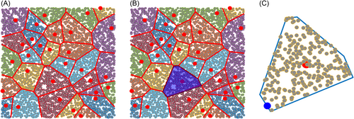
In the cell with the largest error, the point farthest from the center cell in the whole cell is selected to accelerate the cell division process in the entire sample region to achieve a better balance between global prediction and local prediction as shown in Figure 1C.

2.3 Basics of EP

EP-based approach selects a new sample point

based on the current sample

to maximize the information obtained from the Candidate sample set

. The determination basis¹⁹ for selecting new samples is

()

where

is an unit vector, correlation parameters

is the Correlation matrix of the l +n points in sample set X_A =

, …,

. The correlation parameters θ in the correlation matrix

are the same as that of the original Kriging model to makes the new sampling points fit the existing meta-modeling.

2.4 Formulation of CVV-DEP and CVV-EP adaptive sampling strategies

In traditional CV-Voronoi method, a cell is selected according to cross validation, and then the sample point in the cell farthest from the center is selected. It can be observed from Figure 1 that the points with the largest distance from the center point are often located on the corners of the unit. The distance between each corner is not much different, but the selection direction represented by each corner is quite different. Choosing the direction of the corners in adaptive adoption is critical to capture more informative points for the learning process to construct the meta-model. Therefore, the EP is introduced into the existing CV-V method to select the selected unit A point that is farther from the center point and can provide more information. In other words, the CV-V strategy is first used to select the cell with the maximum error and Equations (5a) and (8) are applied to calculate the distance from the center point and the “information content” for all sample points in the selected cell. The “information amount” and the distance of all candidate samples are then normalized by corresponding maximum values. The point with balanced information and distance is selected in the entire unit as follows:

()

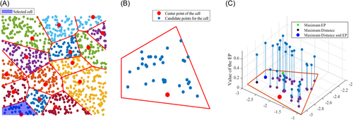
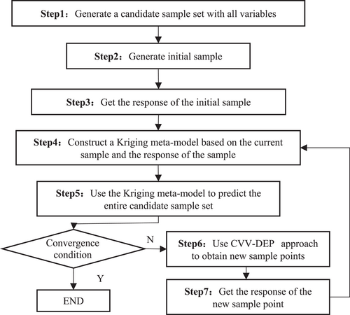
Figure 2 shows the schematics for the CVV-DEP adaptive sampling. It can be observed in Figure 2C that the sample with balanced distance and entropy is not necessarily same as those with maximum entropy or largest distance. Based on the principle of combining CV-V and EP approach, Figure 3 shows the flow chart of CVV-DEP sampling strategy.

3 EVALUATION OF CVV-DEP FOR NONLINEAR FUNCTIONS

To demonstrate the significant advantages of the CVV-DEP adaptive sampling method, six numerical examples are used for verification and comparison. Numerical examples range from simple to complex, including polynomials, exponential functions, trigonometric functions, and their various combinations.

3.1 Nonlinear functions

Six functions are selected to evaluate the effectiveness of the proposed method, which are given as following

F1 function

()

F2 function

()

F3 function

()

F4 function

()

F5 function

()

F6 function

()

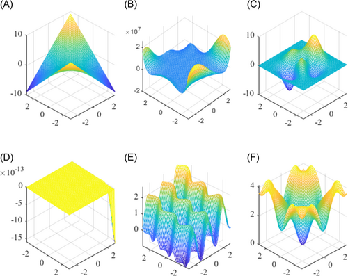
These functions represent different nonlinear behavior as shown in Figure 4. F1 function is a relatively simple binomial. F2 function is a more complex polynomial and is relatively flat in the middle of the entire region with strong nonlinear around. F3 function is relatively flat around and has strong nonlinearity in the middle. F4 function in the whole region is almost zero, but it shows drastic changes in the angle. F5 function has periodic oscillation; F6 function oscillates evenly around and has a low peak in the center.

To better illustrate the sample selection processes for CV-V, CVV-EP, and CVV-DEP, take the F3 function as an example. Assume five initial sample points through Latin hypercube sampling. Figure 5 shows the partition of entire space by initial sample points into five Voronoi cells. For comparison, a total of 10,000 validation points is used to compare the accuracy of Kriging meta-models from different sampling strategies, and RMSE smaller than 0.01 is used as convergence criterion.

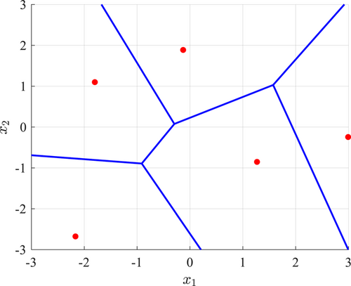
Figure 6 presents the selection process of four additional samples using the proposed adaptive CVV-DEP strategy. For each step, the sample points selected by CV-V and CVV-EP strategies are also included for the purpose of comparison. Figure 6A shows different sample points for largest EP and largest distance. This implies that the CV-V and CVV-EP strategies will lead to different sample point even though same initial sample points are used. The CVV-DEP strategy balances the EP value and the distance which leads to the same point from CV-V. It can also be observed in Figure 6A that the EP value presents a funnel shape around the center point of the Voronoi cell, which has zero EP value is zero. For the second selected sample, the EP value in Figure 6B shows wavy variation for the selected cell with zero at the center point. The sample points selected by all three strategies are the same. Similar observation can be made in Figure 6C as that in Figure 6A, where CV-V and CVV-DEP select the same point but different that from CVV-EP. The variation of EP value in the cell however is observed to be smoother around the center than that observed in Figure 6A. The fourth additional samples selected by three strategies are shown to be different in Figure 6D. The variation of EP value in Figure 6D is observed to continuously change and differ from those in Figure 6A–C. Figure 6 clearly demonstrates the differences between the three CV-based strategies.

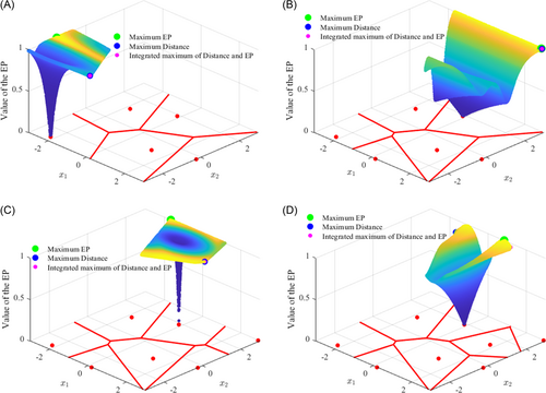
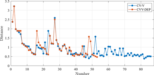
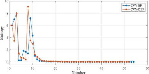
Figure 7 presents the variation of distance between selected sample and the center in the Voronoi cell CVV-DEP and CV-V methods. It is worth noting that the CVV-EP does not utilize the distance for sample selection therefore is not presented. It can be observed that, although CVV-DEP accounts for EP value, but its maximum distance decreases in the same trend as that of CV-V. Under the same convergence criterion, the CV-V strategy has almost same distance as that of CVV-DEP, indicating that the multiple learning times of CV-V eliminates the differences of each selected sample unit, promoted the units of each sample to be more uniform, but reduced the differences of each unit due to the complexity. This is disadvantageous for locally nonlinear functions. As shown in Figure 8 for the variation of EP values of selected samples from CVV-DEP and CVV-EP, it can be observed that CVV-DEP and CVV-EP have almost same decreasing trend of EP values after considering the distance. The EP value and maximum distance of CVV-DEP have the same trend as those of CV-V and CVV-EP considering only one factor, but accounting for both EP and distance helps accelerate the learning process.

For the Kriging meta-models from three strategies after convergence, Figure 9 presents the variation of root-mean-square error (RMSE) for the 10,000 validation points. It can be observed that, despite similar trend as CV-V, CVV-DEP shows much earlier convergence. This implies that CVV-DEP enables less samples for the same accuracy of Kriging meta-model. CVV-EP, on the other hand, shows larger RMSE error than those of the other two but has similar convergence as CVV-DEP.

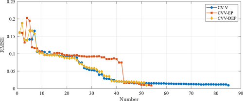
Figure 10 presents the final selected sample points and the partitions of sample space for the three strategies. Similar to Figure 7, CVV-DEP has a more obvious difference in the size of the selected sample unit when compared with CV-V. Compared with the actual image of F3 function in Figure 4, the samples selected by the CVV-DEP strategy are mostly concentrated in the part with relatively strong nonlinearity, while the unit sizes of the samples selected by the CV-V method are relatively uniform.

3.2 Results and discussion

Under the same convergence criterion, the six equations are run three times for each strategy, and the numbers of selected sample points are presented in Table 1. Due to weak nonlinearity, the total number of sample points is relatively small for all three strategies for the F1 function. For the F2 and F3 functions with strong nonlinearity, the total number of sample points decreased significantly for CVV-DEP and slightly for CVV-EP. F4 function has local extreme variation. As can be observed from Table 1, the total number of sample points for CVV-EP decreases a little more than CVV-DEP, indicating that considering EP could improve self-adaptation for function equations with local changes. For the F5 function, CVV-DEP enables effective balance between global expansion and local concentration by considering both distance and EP. F6 function has stronger nonlinearity, where all three strategies are observed to require more sample points than for other functions. The CVV-DEP shows slight better performance than the other two.

Table 1. Results of running times of six functions

Sampling strategy
Functional equation	CV-V	CVV-DEP	CVV-EP
F1 function	9	7	7
	9	8	7
	9	7	8
F2 function	66	57	64
	65	58	61
	67	59	64
F3 function	86	53	55
	77	53	67
	69	52	58
F4 function	52	47	44
	50	35	34
	64	52	45
F5 function	89	79	95
	93	77	96
	88	74	95
F6 function	115	98	106
	108	100	107
	97	93	96

Abbreviations: CV-V, cross validation-Voronoi; CVV-EP, cross validation-Voronoi and entropy; CVV-DEP, cross validation-Voronoi distance and entropy.

4 COMPUTATIONAL SIMULATION OF CVV-DEP FOR HYBRID SIMULATION

Computational simulation is further conducted to evaluate the efficacy of proposed CVV-DEP strategy for hybrid simulation to quantify uncertainty through limited number of laboratory experiments.

4.1 Nonlinear 2-DOF system

A nonlinear 2 degrees of freedom (2-DOF) series system is considered as shown in Figure 11. A similar system was also used by Abbiati & Marelli³⁸ in a numerical benchmark study for adaptive Kriging-based hybrid simulation for structural reliability analysis. The spring connecting the two masses is assumed to be the experimental substructure and has inelastic behavior, while the spring connecting the two masses to the fixed support is linear elastic. For the purpose of computational simulation, the force-deformation relationship of the experimental substructure (i.e., the nonlinear spring) is numerically emulated using the Bouc-Wen model.³⁹ The equations of motion of the 2-DOF system can be expressed as:

()

where

represents the restoring force of nonlinear spring;

and

represents the displacement and velocity;

and

are the mass, damping, and stiffness parameters, respectively;

is the acceleration history of selected ground motion. B uniform modal damping is assumed for the calculation of the damping matrix. The parameters of the 2-DOF system are presented in Table 2. The linear elastic natural frequencies of the 2-DOF system are 1.376 and 2.275 Hz (i.e., the natural periods are 0.727 and 0.440 s).

Table 2. Properties of 2-DOF system

Parameter
Value
Unit				-	-	-	-

The 2-DOF system is assumed to fail when the elongation of the inelastic spring exceeds certain limit value. Thus, the maximum absolute elongation

is defined as the quantity of interest obtained via computational simulation of the 2-DOF system:

()

where u₁ and u₂ are the displacements of the two masses, respectively; and the vector

represents the uncertainty parameters to be considered for stochastic seismic response assessment in this study. Statistic properties of two elastic spring stiffness are listed in Table 3. The ground motions used in the study is selected from a suite of stochastic ground motions generated using the probability model,⁴⁰ where seismic ground motion is derived through time-modulation of a normalized filtered white-noise process with the filter having time-varying parameters. Figure 12 presents the ground motion used for computation simulation.

Table 3. Properties of structural uncertain parameters

Parameter
Range	[2 × 10⁵ 6 × 10⁵]	[5 × 10⁵ 1.5 × 10⁵]
Destitution	Uniform	Uniform

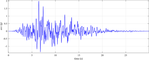
The initial sample points are selected as five and a total of 10,000 validation points are used to evaluate the accuracy of the final Kriging meta-model. The convergence condition is used for RMSE of validation points less than 0.01. To avoid the impact of random sampling, same set of candidate samples is used for all three strategies and a total of three runs are conducted for each strategy. Figure 13 presents the scatter plots of selected sample points to explore the difference in the adaptive sampling process. As can be observed, CVV-DEP has fewer sample points in the middle region with relatively flat response compared with the other two selection methods, and the sample points selected in the region with rapid change are basically the same as those of the other two methods. It shows that CVV-DEP can more effectively identify regions with strong nonlinearity.

Figure 14 presents the comparison between Kriging prediction and actual displacement response for the validation points. It can be observed that, after convergence is reached, all three adaptive strategies show excellent accuracy in Kriging prediction with the values of R² close to 100%.

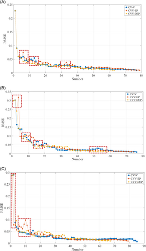
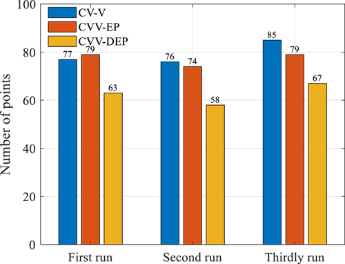
Figure 15 presents the variation of RMSE error for the three runs of adaptive sampling strategies. As can be observed that CVV-EP has greater oscillation than the other two. For the initial stage of the first and second run, single EP value is shown to have an adverse effect on RMSE, while at the initial stage of the third adaptive selection point, the single EP value had a favorable effect. This implies that the initial and candidate sample sets have big influence on the performance of CVV-EP at the early stage of sampling. On the other hand, the decreases of RMSE for CV-V and CVV-DEP are observed to steadier and more stable. Compared with CV-V, the CVV-DEP strategy has almost same decrease of RMSE but faster convergence. The total number of selected sample points are summarized in Figure 16 for all three strategies. As can be observed, CVV-DEP converges faster than both CV-V and CVV-EP.

4.2 Maximum response of single-degree-of-freedom (SDOF) structure with self-centering viscous damper (SC-VD)

The SDOF structure with SC-VD is utilized to further evaluate the capacity of proposed method for global meta-modeling of maximum displacement response under earthquake excitation. The SC-VD device is considered an experimental substructure and the rest is taken as analytical substructure. Chen et al.³⁶ integrated the Co-Kriging technique with real-time hybrid simulation to quantify the effect of structural uncertainty on the same SDOF structure. The newly developed SC-VD device is composed of preloaded ring springs for SC ability and a fluidic VD for energy dissipation.⁴¹ It can be simplified as a parallel connection of a variable stiffness damper and a velocity-dependent VD, where the force–displacement relationship of ring springs can be approximately expressed as:

()

where K₁ and K₂ are the initial and loading axial stiffness of the ring springs, respectively; U is the deformation of the damper; P_a and f_d are the damper preload force and measured restoring force, respectively; C is damping coefficient; and U_g is the internal gap of the damper. The uncertain structural parameters are mass M and stiffness k_E, and their distribution is shown in Table 4. A different ground motion in Figure 17 is used for earthquake excitation.

Table 4. Uncertain parameter distribution of structure

Random variable	Distribution type	Mean	Standard deviation
Mass M (ton)	Gaussian	200	20
Stiffness k_E (N/mm)	Gaussian

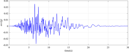
Similarly, three runs of computational simulation are conducted for all three strategies. However, different from previous application, the total number of sample points is set to be 50 to compare the variations in convergence. This is to accommodate the fact that each experimental research often has limited resource and time for laboratory testing. Taking the first run as an example, the final sampling point distribution is shown in Figure 18 for all three strategies.

Integrating EP and distance enables the CVV-DEP to have selected samples scattered more evenly in the beginning stage. Samples from CVV-EP and CV-V however are biased to the right first and then to the left, which might lead to less effectiveness in global exploration. In addition, the aggregation phenomenon of CVV-DEP and CVV-EP samples is more obvious than that of CV-V, and the distance between CV-V samples is relatively uniform. In practical engineering with strong local nonlinearity, CVV-DEP and CVV-EP are better than CV-V in local exploration.

Figure 19 shows the comparison between Kriging prediction and actual maximum displacement responses for validation sample points. Good agreement can be observed and the fitting R² of the three methods are 98.27%, 98.19%, and 97.72%, respectively. This further proves that adaptive sampling using CVV-DEP is more accurate than the other two methods.

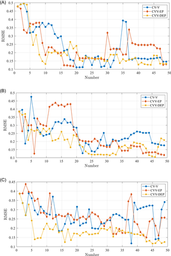
Figure 20 presents the variation of RMSE with the increase of sample points. The beginning three RMSE values are same for CVV-DEP and CV-V, indicating that the two strategies select the same sample points. The CVV-DEP is observed to have more stable decrease in RMSE that both CV-V and CVV-EP.

5 SUMMARY, CONCLUSIONS, AND FUTURE WORK

This study proposes an adaptive sampling strategy to integrate CV-V and entropy approach for global meta-modeling. Cross validation is used to identify the cell with largest error in the Voronoi partition of entire sample space. Both distance and entropy are considered to select the most informative sample in the selected cell. The effectiveness of the proposed CVV-DEP method is first verified through six numerical functions then by computational simulation of hybrid simulation of two systems. The following conclusion can be summarized based on the analysis:

(1)
Different improvement is observed in CVV-DEP for the numerical functions when compared with CV-V and CVV-EP. CVV-EP may require fewer learning sample points than CVV-DEP for functions with local extreme nonlinearity, indicating that adaptative sampling can be more effective when taking entropy into account.
(2)
The EP value and the distance of selected sample points by CVV-DEP have the same trend of decrease as that of CV-V and CVV-EP. Integrating of EP value and distance enables sampling to be more concentrated in the region with strong nonlinearity.
(3)
The distance between the final selected samples from CV-V is relatively uniform, while the aggregation phenomenon of the final selected samples from CVV-DEP and CVV-EP is more obvious implying for the effectiveness of CVV-DEP in identifying regions with strong nonlinearity of functional functions.
(4)
The proposed CVV-DEP demonstrates better efficiency than CVV-EP and CV-V when integrated with hybrid simulation for global modeling of system response. For same convergence, CVV-DEP requires fewer samples than the other two.

In this study, the CVV-DEP adaptive sampling method is applied to the numerical simulation of hybrid simulation. Future research will experimentally evaluate this efficient adaptive sampling strategy to real-time hybrid simulation for uncertainty quantification for more realistic engineering structures. Future will focus on further optimization of adaptive sampling strategies and their experimental assessment.

NOMENCLATURES

: Acceleration history of selected ground motion;
B: Uniform modal damping;
: Damping parameters of the 2-DOF system;
C: Damping coefficient;
: Distance between candidate points and existing sample points;
: Prediction error of the cell;
f_d: Damper measured restoring force;
: Restoring force of nonlinear spring;
: Basis functions of Kriging model;
: Unit vector;
: Stiffness parameters of the 2-DOF system;
K₁ and K₂: Initial and loading axial stiffness of the ring springs;
k_E: Stiffness parameters of SDOF structure;
: Mass parameters of the 2-DOF system;
M: Mass parameters of SDOF structure;
P_a: Damper preload force;
: Correlation matrix of any two sample points and ;
: Correlation matrix for X_A;
: Criteria for selecting sensitive cells;
: Criteria for selection of a new sample by EP method;
: Criteria for selection of a new sample by CVV-DEP method;
: Displacement of the 2-DOF system;
: Maximum absolute elongation;
U: Deformation of the damper;
U_g: Internal gap of the damper;
: Velocity of the 2-DOF system;
x: The input sample;
: The center point of a cell;
: The j^th-dimensional input variable;
: Candidate sample set;
X_A: Union of candidate samples and input samples;
: The response to data points;
: True response of ;
: Predicted value at of the meta-model without ;
: Regression coefficient of Kriging model;
: Correlation parameter of the correlation matrix;
: Predicted mean for sample point x;
: Predicted variance for sample point x.

ACKNOWLEDGMENT

This study effort was supported in part by the Ministry of Science and Technology of the People's Republic of China under Grant No. 2018YFE0206100.

CONFLICTS OF INTEREST

The authors declare no conflicts of interest.

REFERENCES

1Kleijnen JPC. Response surface methodology for constrained simulation optimization: an overview. Simul Model Pract Theory. 2008; 16(1): 50-64.
10.1016/j.simpat.2007.10.001
Web of Science® Google Scholar
2Kleijnen JPC. Kriging meta-modeling in simulation: a review. Eur J Oper Res. 2009; 192(3): 707-716.
10.1016/j.ejor.2007.10.013
Web of Science® Google Scholar
3Ben-Hur A, Horn D, Siegelmann HT, et al. Support vector clustering. J Mach Learn Res. 2001; 2(2): 125-137.
Web of Science® Google Scholar
4Hurtado JE, Alvarez DA. Neural-network-based reliability analysis: a comparative study. Comput Methods Appl Mech Eng. 2001; 191(1-2): 113-132.
10.1016/S0045-7825(01)00248-1
Web of Science® Google Scholar
5Blatman G, Sudret B. An adaptive algorithm to build up sparse polynomial chaos expansions for stochastic finite element analysis. Probabilistic Eng Mech. 2010; 25(2): 183-197.
10.1016/j.probengmech.2009.10.003
Web of Science® Google Scholar
6Fang HB, Horstemeyer MF. Global response approximation with radial basis functions. Optim Eng. 2006; 38(4): 407-424.
10.1080/03052150500422294
Web of Science® Google Scholar
7Jiang C, Qiu H, Gao L, Wang D, Yang Z, Chen L. Real-time estimation error-guided active learning kriging method for time-dependent reliability analysis. Appl Math Model. 2020; 77: 82-98.
10.1016/j.apm.2019.06.035
Web of Science® Google Scholar
8Mooney CZ. Monte Carlo simulation. 116. Sage publications; 1997.
10.4135/9781412985116
Google Scholar
9Iman RL, Davenport JM, Zeigler DK. Latin hypercube sampling (program user's guide). 1980;OSTI 5571631.
Google Scholar
10Sobol IM. Sensitivity estimates for nonlinear mathematical models. Math Model Comput Exp. 1993; 1(4):407414.
Google Scholar
11Jones DR, Schonlau M, Welch WJ. Efficient global optimization of expensive black-box functions. J Glob Optim. 1998; 13(4): 455-492.
10.1023/A:1008306431147
Web of Science® Google Scholar
12Sasena MJ, Papalambros P, Goovaerts P. Exploration of meta-modeling sampling criteria for constrained global optimization. Eng Opt. 2002; 34: 263-278.
10.1080/03052150211751
Web of Science® Google Scholar
13Echard B, Gayton N, Lemaire M. AK-MCS: an active learning reliability method combining kriging and Monte Carlo simulation. Struct Saf. 2011; 33(2): 145-154.
10.1016/j.strusafe.2011.01.002
Web of Science® Google Scholar
14Chen X, Zhang Y, Zhou W, Yao W. An effective gradient and geometry enhanced sequential sampling approach for kriging modeling. Struct Multidiscipl Optim. 2021; 64(6): 3423-3438.
10.1007/s00158-021-03016-9
Web of Science® Google Scholar
15Jin RC, Chen W, Sudjitanto A. On sequential sampling for global meta-modeling in engineering design. Proceedings of the ASME 2002 International Design Engineering Technical Conferences and Computers and Information in Engineering Conference (Paper No: Detc2002/DAC-34092), September 29-October 2, 2002; 2002: 539-548.
Google Scholar
16Crombecq K, Gorissen D, Deschrijver D, Dhaene T. A novel hybrid sequential design strategy for global surrogate modeling of computer experiments. SIAM J Sci Comput. 2001; 33(4): 1948-1974.
10.1137/090761811
Web of Science® Google Scholar
17Xu S, Liu H, Wang X, Jiang X. A robust error-pursuing sequential sampling approach for global meta-modeling based on voronoi diagram and cross validation. ASME J Mech Des. 2014; 136(7):071009.
10.1115/1.4027161
Web of Science® Google Scholar
18Shannon CE. A mathematical theory of communication. Bell Syst Tech J. 1948; 27(3): 379-423.
10.1002/j.1538-7305.1948.tb01338.x
Web of Science® Google Scholar
19Currin C, Mitchell T, Morris M, Ylvisaker D. Bayesian prediction of deterministic functions, with applications to the design and analysis of computer experiments. J Am Stat Assoc. 1991; 86(416): 953-963.
10.1080/01621459.1991.10475138
Web of Science® Google Scholar
20Dermitzakis SN, Mahin SA. Development of substructuring techniques for on-line computer controlled seismic performance testing. Report UCB/EERC-85/04, Berkeley: Earthquake Engineering Research Center, University of California; 1985.
Google Scholar
21Nakashima M. Hybrid simulation: an early history. Earthq Eng Struct D. 2020; 49(3): 949-962.
10.1002/eqe.3274
Web of Science® Google Scholar
22Wang T, Cheng C, Guo X. Model-based predicting and correcting algorithms for substructure online hybrid tests. Earthq Eng Struct D. 2012; 41(15): 2331-2349.
10.1002/eqe.2190
Web of Science® Google Scholar
23Yang Z, Tian Y, Zhou T, et al. Reinforcement learning control method for real-time hybrid simulation based on deep deterministic policy gradient algorithm. Struct Control Health Monit. 2022; 26: 4880-4891.
Google Scholar
24Wang Z, Ning X, Xu G, Zhou H, Wu B. High performance compensation using an adaptive strategy for real-time hybrid simulation. Mech Syst Signal Process. 2019; 133:106262.
10.1016/j.ymssp.2019.106262
Web of Science® Google Scholar
25Zhong W, Chen Z. Model updating method for hybrid simulation based on global sensitivity analysis. Earthq Eng Struct D. 2021; 50(14): 3792-3813.
10.1002/eqe.3533
Web of Science® Google Scholar
26Wu B, Ning X, Xu G, Wang Z, Mei Z, Yang G. Online numerical simulation: a hybrid simulation method for incomplete boundary conditions. Earthq Eng Struct D. 2018; 47(4): 889-905.
10.1002/eqe.2996
Web of Science® Google Scholar
27Mei Z, Wu B, Bursi OS, et al. Hybrid simulation with online model updating: application to a reinforced concrete bridge endowed with tall piers. Mech Syst Signal Process. 2019; 123: 533-553.
10.1016/j.ymssp.2019.01.009
Web of Science® Google Scholar
28Ozdagli AI, Xi W, Ou G, et al. Experimental verification of an accessible geographically distributed real-time hybrid simulation platform. Struct Control Health Monit. 2019; 27(2):e2483.
Web of Science® Google Scholar
29Zhou H, Wang T, Du C, Chen C. Multi-degree-of-freedom force-displacement mixed control strategy for structural testing. Earthq Eng Struct D. 2020; 50(2): 354-374.
10.1002/eqe.3334
Web of Science® Google Scholar
30Du C, Wang T, Qie Y, Marino E, Zhou H. Staggered coordination in substructure online hybrid test on a RC frame retrofitted by BRBs. Bull Earthq Eng. 2019; 17(7): 4141-4167.
10.1007/s10518-019-00636-x
Web of Science® Google Scholar
31Qie Y, Barbagallo F, Marino EM, Du C, Wang T. Full-scale hybrid test for realistic verification of a seismic upgrading technique of RC frames by BRBs. Earthq Eng Struct D. 2020; 49(14): 1452-1472.
10.1002/eqe.3312
Web of Science® Google Scholar
32Tao JP, Charlson ES, Zhu Y, et al. Real-time hybrid simulation of high-speed train-track-bridge interactions using the moving load convolution integral method. Eng Struct. 2021; 228: 35-46.
Web of Science® Google Scholar
33Tsokanas N, Zhu X, Abbiati G, Marelli S, Sudret B, Stojadinović B. A global sensitivity analysis framework for hybrid simulation with stochastic substructures. Front Built Environ. 2021; 7:778716.
10.3389/fbuil.2021.778716
Google Scholar
34Ligeikis C, Christenson R. Identifying stochastic frequency response functions using real-time hybrid substructuring, principal component analysis, and kriging metamodeling. Exp Tech. 2020; 44(6): 763-786.
10.1007/s40799-020-00389-2
Web of Science® Google Scholar
35Yu G, Chen C, Hou H, Chen M, Zhang R. Experimental evaluation of CV-Voronoi based adaptive sampling for kriging meta-modeling of multiple responses through real-time hybrid simulation. Earthq Eng Struct D. 2022; 51(8): 1943-1961.
10.1002/eqe.3646
Web of Science® Google Scholar
36Chen C, Yang Y, Hou H, Peng C, Xu W. Real-time hybrid simulation with multi-fidelity Co-Kriging for global response prediction under structural uncertainties. Earthq Eng Struct D. 2022; 51: 2591-2609.
10.1002/eqe.3690
Web of Science® Google Scholar
37Lophaven SN, Nielsen HB, Søndergaard J. Dace: a Matlab Kriging toolbox, version 2.0. 2002.
Google Scholar
38Abbiati G, Marelli S. Sequential experimental design of hybrid simulations for Bayesian calibration of computational simulator. Proceedings of 17th World Conference on Earthquake Engineering, Sendai, Japan, September 13-18, 2020;2020.
Google Scholar
39Smail M, Fayçal I, Rodellar J. The hysteresis Bouc-Wen model, a survey. Arch Comput Methods Eng. 2009; 16(2): 161-188.
10.1007/s11831-009-9031-8
Web of Science® Google Scholar
40Rezaeian S, Kiureghian AD. Simulation of synthetic ground motions for specified earthquake and site characteristics. Earthq Eng Struct D. 2010; 39(10): 1155-1180.
10.1002/eqe.997
Web of Science® Google Scholar
41Zhu R, Guo T, Mwangilwa F. Development and test of a self-centering fluidic viscous damper. Adv Struct Eng. 2020; 23(13): 2835-2849.
10.1177/1369433220920464
Web of Science® Google Scholar

Volume1, Issue3

September 2022

Pages 350-370

This article also appears in:

Hybrid Simulation and Dynamic Tests

A cross validation-Voronoi and entropy based adaptive sampling strategy for uncertainty quantification through hybrid simulation

Abstract

1 INTRODUCTION