Research on numerical solution algorithm for real-time hybrid simulation of high-speed railway on suspension bridge

1 INTRODUCTION

With the rapid development of high-speed railways in China, the number of railway bridges such as suspension bridges is increasing. Suspension bridge is a typical flexible structure, which will produce large static deformation and dynamic response under gravity load, train dynamic load, and temperature,^1-3 and when the train is running, the coupling vibration of the train-bridge poses a great challenge to the smoothness of the train. Therefore, the study of the smoothness of high-speed trains on long-span suspension bridges under different conditions is a key issue. At the same time as the theoretical research, corresponding tests need to be carried out to verify the dynamic responses such as the vibration of the train and bridge. Field testing requires a lot of financial resources, and on-site measurement when the reliability of the bridge structure and control system cannot be guaranteed, which will cause a waste of human resources or even danger, so it is necessary to develop test methods in the laboratory.

Real-time hybrid simulation (RTHS) combines the advantages of numerical simulation and experimental test, the requirements for the capacity of the specimen and the output of the loading system are low and can reflect the time rate correlation of the specimen, so it is widely used in the power test of building structures, bridge structures, and bridges. In RTHS, the part with a clear constitutive relationship, easy to simulate or not easy to test usually seems as a numerical substructure, and components with strong nonlinearity and unclear physical characteristics (such as dampers) are tested as physical substructures, and the dynamic analysis of the system is realized through the real-time interaction of the data between the numerical substructure and the experimental substructure. In 2013, Terzic and Stojadinovic⁴ studied the postseismic traffic performance of the viaduct using the pier as a test substructure and applied a vertical load to the pier to simulate truck load. Data obtained from these tests suggest that a typical California overpass has the ability to carry heavy truck loads immediately after a major earthquake.⁵ To solve the control problem of high-frequency signals, an adaptive time series (ATS) compensation algorithm combining linear secondary Gauss is applied to the vehicle-rail-bridge structure, and real-time hybrid experiments are performed. Guo et al.⁶ used the X-PC platform to establish a real-time hybrid test architecture to study the driving safety of high-speed rail bridges after the earthquake, in which the bridge-track as a numerical substructure was solved using MLSA in the test.

The integration algorithm is important in the RTHS to solve the structural equation of motion, to ensure calculation efficiency, the integration algorithm should have sufficient accuracy and stability.^{7, 8} In the RTHS, the real-time calculation result of the numerical substructure determines the drive control signal of the next-step loader, which has high requirements on the calculation time of each step of the solution, and the calculation efficiency of the integration algorithm determines the scale and complexity of the structure system.⁹ Therefore, when applying traditional numerical integration algorithms to RTHS, it is necessary to consider not only the solution time but also the control of the loader (displacement and speed). In recent years, many scholars have carried out a series of research around RTHS solution algorithms and achieved fruitful results. The Newmark series of algorithms¹⁰ include explicit Newmark algorithms, linear acceleration methods, and so forth, which assumes of acceleration changes and have good accuracy and stability, which has strong reference significance. Wu et al.^{7, 11} applied the central difference method and OSM algorithm to the RTHS of sharing a degree of freedom system to explore the applicability of the two algorithms, and the numerical research results show that the accuracy and stability of the center difference method and the OSM algorithm in the RTHS have decreased. Zhu et al.^{12, 13} conducted a stability study of the KR algorithm in the RTHS of multiple degrees of freedom (DOF) through discrete control theory and conducted stability analysis of many classical integral algorithms (proposed before 2015) in the same way the following year. Verma et al.¹⁴ considered the damping force in the RTHS and carried out the study of the characteristics of four explicit integration algorithms under this working condition, and the results showed that the damping ratio of the experimental substructure would affect the accuracy and stability of the algorithm. When the damping ratio increased, it was easier to maintain the stability of the integration algorithm, but the accuracy of the algorithm would be lost. Based on the Newmark series algorithm, Chang et al.¹⁵ introduced the adjustment parameter γ and β into the previously proposed Chang-2002¹⁶ algorithm, and proposed a display algorithm with the same numerical characteristics as the Newmark series algorithm.

The numerical substructure in the RTHS requires that the integration algorithm has sufficient efficiency and stability to meet the requirements, and the explicit stepwise integral algorithm is generally used in RTHS. However, for numerical models with high complexity, such as long-span suspension bridge-train coupling models, which have tens of thousands of DOF, it is difficult for existing integration algorithms to meet the real-time requirements of RTHS.

Recently, scholars have proposed a large number of structural response prediction models based on neural networks. Compared with the traditional stepwise integral solution method, the network model can significantly improve the computational efficiency and reduce the computational cost, making the neural network have great advantages in predicting the nonlinear response of the structure. Ok et al.¹⁷ used artificial neural networks (ANNs) to fit the bridge response caused by vehicle loads and successfully obtained an estimated bridge displacement time course curve. Chakraverty et al.¹⁸ proposed to use the adaptive model for the prediction of the nonlinear behavior of the structure caused by earthquakes, and the results showed that in the dynamic analysis, ANN can accurately predict the structural response of the PBD framework, and the calculation time is greatly reduced compared with the traditional solution algorithm. To predict the failure time of reinforced concrete structures, Chatterjee et al.¹⁹ and Sankhadeep et al.²⁰ proposed a method to detect the possibility of future failure of multilayer steel-concrete structure based on multilayer perceptions and the neural network particle swarm algorithm classifiers, respectively. Zhang et al.²¹ trained on available datasets by long-short-term memory (LSTM) ANNs to accurately predict the elastic and inelastic responses of building structures. Xu et al.²² proposed a recursive LSTM for predicting the seismic response of nonlinear structures at arbitrary lengths and sampling rates, and the final results showed that the proposed network model can fully reproduce the local and global characteristics of four different structural time-course response datasets, with good accuracy and generalization ability. LSTM as a variant of a neural network is designed to capture long-term data correlations for modeling sequence data. The strict time-dependent nature of structural response sequences makes LSTM ideal for neural network architectures, and LSTM's structure and unique gating mechanism perfectly simulate implicit integral solutions.²³

In this paper, the LSTM is applied to RTHS as a numerical substructure to evaluate its stability, accuracy, and real-time performance in the test, and the effectiveness of the analysis of the dynamic response of the suspension bridge-train system by RTHS is verified. A semi-active suspension-train-suspension bridge coupling RTHS framework is constructed, in which the train-suspension bridge part is replaced by LSTM. The prediction performance of the network models is evaluated through time course comparison, regression analysis, and normalization error distribution, and the feasibility of neural networks instead of numerical substructures in RTHS is analyzed.

2 RTHS FRAMEWORK

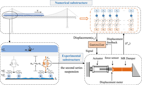
As shown in Figure 1, the first step of RTHS inputs the damping force F_ss of the first time to the neural network, and the network calculates the dynamic response of the train when crossing the bridge at this time. Through the data transmission system, the relative displacement of bogie and the car body (i.e., the amount of suspension compression of the second series u_ss) of this time step is transmitted to the controller, and the controller sends the u_ss to the actuator. After the loading is completed, the damper feeds back the secondary suspension force F_ss measured by the force sensor to the neural network and calculates the output of numerical substructure in the next time step.

2.2 Virtual RTHS

In this paper, the method of simulation model²⁵ is used to establish an actuator model, and the model performance index is derived from the servo hydraulic actuator system of the National Engineering Research Center for High-speed Railway Construction Technology of Central South University as shown in Figure 2, and its transfer function is shown in Equation (3), where x_r is the actual displacement of the actuator, and x_c is the target displacement of the controller.

$$()

Utilizing the ATS compensator method,²⁶ the compensated input actuator displacement command u_c is expressed at time t_k as:

$$()

$$()

Considering the scale effect and test cost, suspended by the secondary suspension of the train is selected as the test substructure. The numerical substructure is the train-suspension bridge system. The numerical substructure calculates the response of the train-bridge system according to the external input excitation and the force feedback F_SS of the virtual physical substructure; the relative displacement $$ of the secondary suspension obtained by the solution is calculated and the time-delay is compensated, the compensated displacement command u_ss is sent to the actuator, the actuator after obtaining the drive command to load the physical substructure, to obtain the damper under the drive signal force feedback F_SS, which feeds it back to the numerical substructure for the next time step. The experimental substructure is a modified Dahl model,²⁷ as shown in the following equation:

$$()

$$()

where $$ is the stiffness coefficient, $$ is the viscosity damping coefficient, $$ is the Coulomb friction related to the current strength, x the damper displacement, $$ is the initial force size; z is the dimensionless hysteresis constant, where σ is the fitting parameter that controls the hysteresis curve.

The dynamic equation for the numerical substructure in RTHS can be expressed by Equation (8). Where the subscripts v and b indicate the train subsystem and the bridge subsystem respectively, and M, C, and K are mass matrix, damping matrix, and stiffness matrix of the structure; $$, $$, and $$ are acceleration, velocity and displacement vectors, respectively. F_v and F_b are the external load vectors of the vehicle subsystem and the bridge subsystem, respectively. F_ss is the force at the interface between the numerical substructure and the experimental substructure, that is, the interaction force between the secondary suspension and the train. Among them, the M, C, K of the train and bridge can be directly derived from the finite element model, which is a definite value and does not change with the change of the incentive size.

$$()

3 DATA SET GENERATION AND PREPROCESSING

In this paper, the bridge analyzed is a double track railway ground anchored suspension bridge, and the center distance between the two lines is 5 m. The elevation of suspension bridge is shown in Figure 3. Its span is (98 + 660 + 98) m. the main tower adopts a reinforced concrete portal frame structure. The bridge tower is of the unequal tower height, and the tower heights on the left and right banks are 196 and 156 m, respectively. The anchoring form is a tunnel anchor. The anchoring length on both banks is 80 m and the inclination angle is 35°.

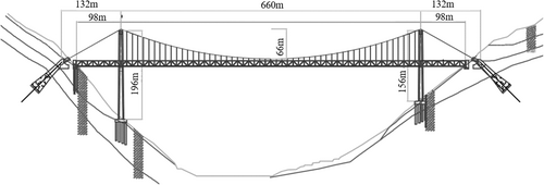
The main span is suspenders with a spacing of 12.2 m, and space cables are used for the side span. The sag of the main cable is 66 m, the rise span ratio is 1/10, and the diameter is 756 mm. The stiffening beam is a deck steel truss with a truss height of 12 m and a truss width of 25 m. The main span section is 12.2 m. The contact point between the stiffening beam and the bridge tower crossbeam is only provided with vertical and horizontal bridge direction bearings, and there is no restriction along the bridge direction. The two ends of the stiffening beam only restrict the displacement in the vertical and horizontal bridge directions. At the same time, a flexible central buckle is added at the mid span of the main span to delay the occurrence of longitudinal drift of the structure.

Materials and section characteristic parameters of main stressed members are given in Table 1.

CRH380a is selected in this study. A single train consists of a body with 5 DOF, including three-way translation and two-way rotation, two bogies (2 × 5 DOFs), and four wheel sets (4 × 6 DOFs), 31 DOFs for a single train. The above three parts are rigid bodies. Damping and linear springs are used to connect the parts. The wheel set does not consider the rotation around the Y-axis. The other rigid bodies have vertical and horizontal translational DOF and rotational DOF around the X-axis, Y-axis, and Z-axis. The definition of DOF of a single train is shown in Table 2. The three views of the train model are shown as Figure 4.

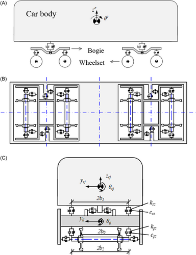
Values of geometric and physical parameters of train components are shown in Table 3.²⁸

Derived from RHTS equation of motion Equation (1), The interaction force between the secondary suspension and the train, which is the change in the dynamic response of the train caused by the external excitation, should be one of the inputs of the network during training. In addition, track unevenness which consist of short wave irregularity and temperature load is the internal excitation that affects the overall structural response, and should also be the input of the network. The relative displacement of the train secondary suspension, the vertical acceleration of the body, the speed of the body, and the speed of the bogie are the output of the network. In summary, the LSTM has an input feature of 2 and an output feature of 4.

In this paper, the main variables affecting the vibration amplitude and characteristics of the train are temperature load, secondary suspension damping coefficient, and train speed. A total of 9 temperature load levels, 15 secondary suspension coefficient grades, and 1 speed class were selected, and the data set contained a total of 135 working conditions. Because the temperature load is included in the track irregularity, the change of damping coefficient is considered when calculating the suspension force, and this paper concentrates on the maximum speed of 250 km, so these parameters do not need to selected as the input of LSTM.

As a result, the training set contains 50 samples, the validation set contains 15 samples, and the test set contains 70 samples.

The response time history of the train from the road bridge transition section before entering the upper bridge to the road bridge transition section after leaving the lower bridge is selected as the sample, and the sampling frequency is 500 Hz.

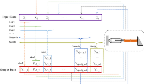
The prediction process of LSTM is shown in Figure 5. In the figure, $$ is the excitation of the k-th time step, and the output of the k-th time step is $$, where $$, t is the total length of the excitation time history, $$ and $$ are the type and quantity of input and prediction time history data, respectively. The excitation is the damping force and irregularity excitation in the secondary suspension of the train, and the output $$ is the nodal angle of the car body, the acceleration of the car body, and the relative displacement between the bogie and the car body. The output dimension of each time step is $$, but only the value of structural dynamic response $$ is input to the physical substructure, and the output of the physical substructure is added to the input of the next time step numerical substructure. For example, the excitation Step1 = (x₁) of the first step, the output response out1 = ($$) of the first step is obtained through LSTM prediction. Set the relative displacement value of the secondary suspension in y_{s1_1} is input to the controller as a command signal. After the experimental substructure is loaded by the actuator, the measured secondary suspension force x₂ is fed back to the LSTM through the force sensor. At this time, the input of the second time step network is Step2 = (x₁, x₂). This completes a recursive step.

4 DYNAMIC RESPONSE PREDICTION

The training set is fed into the LSTM model, the data of the validation set is used to select reasonable parameters for the network, and then the trained network model is used to replace the numerical substructure in RTHS to predict the time course of the train dynamics response when running on the large span suspension bridge. The prediction results are evaluated and analyzed by training set to test the prediction performance of the established neural network model on the nonlinear response of the structure.

To study the predictive performance of the LSTM model for the nonlinear structural response of the train-bridge system, the model output of the model responds to the compression amount of the secondary suspension of the train, through the time curve, Pearson correlation coefficient²⁹ and normalization error analysis³⁰ are analyzed and evaluated on three criteria.

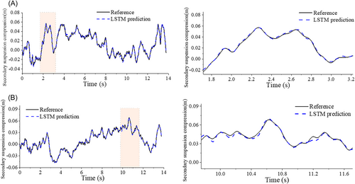
First, the LSTM model is used to predict the response time course of the suspension compression of the second series of trains, and Figure 6 shows the comparison of the predicted values of the two samples in the test set with the reference value time course curve, of which Figure 6A is the cooling 21°C, secondary suspension damping 12 k working condition, Figure 6B is the temperature rise of 21°C, the secondary suspension damping 17.5 k working condition. In this section, the response calculated by SIMPACK was selected as a reference value. Zooming in on the curves of the two samples at the peak, as shown on the right side of Figure 6, the two curves change the trend consistently, and the prediction results of the network model for the above samples are in good agreement with the reference values.

To determine the degree of correlation between the prediction results of the network model and all the test samples, the regression analysis of the results was performed, and the correlation coefficient of LSTM for the prediction results of all samples was above 0.9, and most of them were above 0.95. In addition, at the confidence interval (CI) [−10%, 10%] of the normalization error o, the confidence level CI of the LSTM is 97%; at the CI [−5%, 5%] of the normalization error the confidence level CI is 90%.

5 RTHS RESULT ANALYSIS

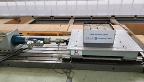
To assess the real-time and accuracy of the LSTM model predicting the dynamic response of the train in the RTHS, the neural network model was used as a numerical substructure, and the semi-active suspension device was simulated as an experimental substructure by the elastic damper model for a virtual real-time hybrid test.

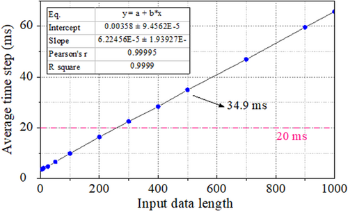
Figure 7 compares the relationship between the length of the network input data and the real-time performance, which is presented by average step time. It can be seen from Figure 7 that the average step time of the LSTM model is approximately proportional to the length of the data input. The time cost inevitably increases with the enlarge of the dimension of the input data. When the data dimension is lower than [2 × 260], the average step time is less than 20 ms. When the data dimension is [2 × 500], the average step time is 34.9 ms. However low dimension of the input data usually leads to low accuracy of the model. As a result, it is faced with the trade-off between the prediction accuracy and the real-time performance of the test in the actual test. To meet the requirements of real-time computing, when the data dimension exceeds [2 × 260], the front part of the input data that has little impact on the later time history prediction results was truncated. For example, when the input data is $$, the input data will be truncated to $$.

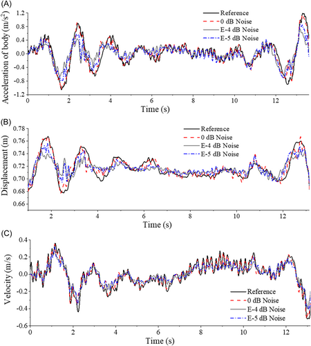
To study the accuracy and the stability of the numerical substructure of the LSTM in the RTSH, the ideal test situation with the LSTM numerical substructure and the RTSH with the noise is compared. The acceleration time history of the car body, the time history of the secondary suspension compression, and the velocity history of the train was analyzing through the peak error under different working conditions. As shown in Figure 8, all operating conditions are cooled by 27°C and the SH magneto-rheological control algorithm is used. The peak acceleration at no noise (0 dB) has better prediction accuracy than the pure numerical simulation results (Reference), with a maximum error of 0.036 and a maximum error rate of 3.03%. Under noise-free conditions, the prediction of the suspension displacement and body speed of the second series has a small error.

6 CONCLUSION

In this paper, LSTM is applied to the coupling vibration study of the train-bridge system, and an RTHS framework for semi-active vibration damping device-train-suspension bridge coupling is established to illustrate the test logic and feasibility, and a dynamic response solution method of numerical substructure based on LSTM is proposed. Then, the feasibility of the network models in RTHS was analyzed, and the predicted performance of the trained network models was evaluated by time course comparison, regression analysis, and normalized error distribution. Finally, the LSTM was applied to a train-bridge RTHS, verify its accuracy and real-time performance. The main conclusions are as follows: it is feasible to use the secondary suspension as the experimental substructure, the train-suspension bridge system as the numerical substructure, and solve it by the LSTM model. The simulation results show that the neural network numerical substructure has good prediction performance for the nonlinear structural response of the train-bridge system. The solution method proposed in this paper can improve the accuracy and efficiency of the numerical substructure of the semi-active damping device-train-suspension bridge RTHS effectively.

CONFLICTS OF INTEREST

The authors declare no conflicts of interest.