Funding information: Gobierno del Principado de Asturias, FC-GRUPIN-IDI/2018/000193; FC-GRUPIN-IDI/2018/000226; Ministerio de Ciencia e Innovación, RTI2018-098085-B-C44; PID2020-119082RB-C22; Ministerio de Economía y Competitividad, MINECO-16-TEC2015-67387-C4-3-R; MTM-2017-83506-C2-2-P

About

Sections

PDF

Tools

Share a link

Email
Wechat
Bluesky

Abstract

The security of a broad family of coding-based cryptographic techniques relies on the hardness of the Syndrome Decoding Problem (SDP). In this problem, the aim is to find a word with a given syndrome and of Hamming weight smaller than a prefixed bound. If this last condition is replaced by “of minimum weight,” then we have the Coset Leader Problem (CLP), being Finding Low Weight Codewords (FLWC) a particular case (when the zero syndrome is considered). An algorithm that has been proposed in order to obtain approximate solutions of problems of these kind (NP-complete) is the Quantum Approximate Optimization Algorithm (QAOA), a variational hybrid quantum-classical algorithm. In this paper, we apply the QAOA to the CLP for binary linear codes. We model the problem, make the theoretical analysis the case of the first level, and introduce some experiments to test its performance. The experiments have been carried out on quantum computer simulators with codes of different lengths and QAOA of different depth.

1 INTRODUCTION

The security of a broad family of coding based cryptographic techniques relies on the hardness of the Syndrome Decoding Problem (SDP). In this problem, given natural numbers $n, k$ , and w such that $k, w \leq n$ , and a parity-check matrix $H \in ℳ_{(n - k) \times n} (𝔽_{2})$ of a binary linear code $(𝔽_{2} = {0, 1})$ , and a syndrome vector $s \in 𝔽_{2}^{n - k}$ , the aim is to find a word $e \in 𝔽_{2}^{n}$ with syndrome $s = H e^{t}$ , of Hamming weight $w t (e)$ smaller than w.¹ In cryptography, for instance, the interest is on random binary linear codes of code rate $\frac{k}{n} \approx 0.5$ , and w slightly higher than the Gilbert–Varshamov bound.² Other case of interest is when the code is a binary Goppa code of coding rate $\frac{k}{n} = 0.8$ , and the weight bound is taken as $⌈\frac{n}{5 \log_{2} n}⌉$ , as the Classic McEliece cryptosystem, as submitted to the NIST Post-Quantum Cryptography standardization process relies on Reference 3.

When the condition $w t (e) \leq w$ of the SDP is replaced by “e of minimum weight,” then we have the Coset Leader Problem (CLP), that is, finding a word of minimum weight among those having the same syndrome s. A particular case of this problem is Finding Low Weight Codewords (FLWC), when the zero syndrome is considered. The decision version of these problems is known to be NP-complete,⁴ hence their importance from the cryptographic point of view. Also, the problem remains difficult when the binary code is randomly chosen and w is taken close to the Gilbert–Varshamov bound.⁵ Other concrete instances such as the ones mentioned above based on binary Goppa codes, are apparently hard too.

Because of this computational hardness, Quantum Computers (QC) are not believed to be able to solve these problems in polynomial time.⁶ However, it might occur that the solution to some instances of these problems could be approximated by a quantum computation technique. One of the proposals in this direction is the Quantum Approximate Optimization Algorithm (QAOA), a variational hybrid quantum-classical algorithm introduced in 2014.⁷ Originally applied to one particular NP-complete problem (MaxCut), this algorithm combines the power of classical minimization of certain parameters and the power of discrete time evolution of QC based on such parameters. Because of its apparent quantum error robustness, it has become a promising candidate to use in the NISQ (Noisy Intermediate-Scale Quantum) era, that is, with a-few-hundred-qubit quantum-error-nonfree QC.

In this paper, we apply the QAOA to the CLP for binary linear codes. This is not the first time that QAOA has been considered in the context of coding theory. In Reference 8, a maximum likelihood channel decoding methodology based on QAOA was proposed. In our paper, we follow some of the ideas introduced there but taking into account the hamming weight of the solutions. This yields to a framework in which a new Hamiltonian models the problem, in the sense that finding minimizing states corresponds to solutions of the posed instance. This is accomplished in the second section of the paper, which also contains background on the QAOA algorithm. Next, we introduce some experiments to test the performance of the QAOA methodology, not only of the first level, but also of levels $p = 1$ –5. For the experiments we have selected the smallest instances of the SDP for random binary linear codes and for the Goppa–McEliece setting contained in the site https://decodingchallenge.org, a webpage devoted to assess the practical hardness of problems in coding theory. Conclusions and future work are given in the final section of the paper.

2 QAOA FOR CLP

Adiabatic quantum computation is a polynomially equivalent model to the standard gate model of quantum computation^{9, 10} that has been applied to solving $N P$ -complete problems.¹¹ Its theoretical foundation is the Quantum Adiabatic Theorem¹² that states, roughly speaking, that if a quantum system is prepared in the ground state of an initial Hamiltonian $H_{I}$ , and that if the system is driven by a sequence of slightly changing Hamiltonians of the form ${\{H (t) = (1 - \frac{t}{T}) H_{I} + \frac{t}{T} H_{F}\}}_{0 \leq t \leq T}$ then, if T is sufficiently large, the final state will be also in the ground state of the final Hamiltonian $H_{F}$ .¹³ In order to solve an $N P -$ complete problem, a final Hamiltonian is introduced, so that its ground states encode its solutions. These solutions are achieved from the evolution of an easy-to-prepare ground state of an initial Hamiltonian, according to the time-dependent Hamiltonian mentioned above.

The evolution of an adiabatic computation can be approximated by the Suzuki–Trotter decomposition.¹⁴ In the particular case of a problem of minimization of a cost function

C : 𝔽_{2} \to ℝ

, a Trotterization of the adiabatic process consists in a alternating sequence of the operators

U (H_{C}, γ_{j}) = \exp (- i γ_{j} H_{C}), U (B, β_{j}) = \exp (- i β_{j} \sum_{l = 1}^{n} X_{l}),

where

H_{C}

is seen as the final Hamiltonian on a quantum space of n qubits with computational basis

{\{| e ⟩\}}_{e \in 𝔽_{2}^{n}}

X_{i}

is the X Pauli operator on the ith qubit, and

γ_{j}, β_{j} \in [0, 2 π]

(1 \leq j \leq p)

are arbitrary angles. The number p determines the depth level of the approximation. This is, in essence, the QAOA, where the initial state is is chosen to be

| ϕ ⟩ = | + ⟩^{\otimes n}

, and the final state is

| γ, β ⟩ = U (B, β_{p}) U (H_{C}, γ_{p}) \dots U (B, β_{1}) U (H_{C}, γ_{1}) | ϕ ⟩

It can be shown that, if

F_{p} (γ, β) = ⟨ γ, β | C | γ, β ⟩

denotes the expected value of C in the final state

| γ, β ⟩

, then

\lim_{p \to \infty} \max_{γ, β \in [0, 2 π]} \{F_{p}\} = \max_{e \in 𝔽_{2}^{n}} C (e) .

In the case of the CLP we want to minimize

w t (e)

among those

e \in 𝔽_{2}^{n}

given syndrome

s = H e^{t}

(we are given natural numbers

n, k,

and w such that

k, w \leq n

, and a parity-check matrix

H \in ℳ_{r \times n} (𝔽_{2})

of a binary linear code, and a syndrome vector

s \in 𝔽_{2}^{r}

, where

r = n - k

). Consequently, we will introduce the cost function

C (e) = w t_{H} (e) + Π d_{H} (s, e H^{t}),

where

d_{H}

is the Hamming distance between the vectors

e H^{t}

and s (i.e., the number of positions in which they differ),

w_{t}

is the Hamming weight of the vector e (i.e., the Hamming distance between the vector e and the zero vector) and

Π

is a penalty introduced to force that the minimal e satisfies the equality

e H^{t} = s

(i.e.,

d_{H} (s, e H^{t})

). The choice of

Π = n + 1

is optimal, as the following result shows.

Proposition 1.Let n and k be natural numbers with $k \leq n$ , let $H \in ℳ_{r \times n} (𝔽_{2})$ be a parity-check matrix of a binary linear code, and let $s \in 𝔽_{2}^{r}$ be a syndrome vector ( $r = n - k$ ). Let us define $C (e) = w t_{H} (e) + Π d_{H} (s, e H^{t})$ , for all $e \in 𝔽_{2}^{n}$ . If $Π \geq n + 1$ , and e is any vector such that $e H^{t} = s$ , then $C (f) > C (e)$ , for all $f \in 𝔽_{2}^{n}$ such that $f H^{t} \neq s$ . On the other hand, if $Π \leq n$ , then there exists a parity-check matrix $H \in ℳ_{r \times n} (𝔽_{2})$ , a syndrome $s \in 𝔽_{2}^{r}$ , and two vectors $e, f \in 𝔽_{2}^{n}$ such that $e H^{t} = s$ , $f H^{t} \neq s$ , but $C (f) \leq C (e)$ .

Proof.For the first part we have $C (f) = w t_{H} (f) + Π d_{H} (s, f H^{t}) \geq 0 + (n + 1) \cdot 1 > n + (n + 1) \cdot 0 = w t_{H} (e) + Π d_{H} (s, e H^{t}) = C (e)$ since $f H^{t} \neq s$ makes $d_{H} (f H^{t}, s) \neq 0$ , and $f H^{t} = s$ gives $d_{H} (e H^{t}, s) = 0$ .

On the other hand, if $Π \leq n$ , then take $H = (1 \dots 1) \in ℳ_{1 \times n} (𝔽_{2}), s = (1) \in 𝔽_{2}$ , $e = (1 \dots 1), f = (0 \dots 0) \in 𝔽_{2}^{n}$ . Then, $C (f) = w t_{H} (f) + Π d_{H} (s, f H^{t}) \leq 0 + n \cdot 1 = n + Π \cdot 0 = w t_{H} (e) + Π d_{H} (s, e H^{t}) = C (e)$ .

Next, we introduce the Hamiltonian related to the cost function C, in the sense that any ground state $| e ⟩$ of $H_{C}$ corresponds to a vector minimizing the function C. The weight function $w t_{H} (e)$ can be written as $\sum_{i = 1}^{n} e_{i}$ , that can be translated into the addition $- \sum_{ν = 1}^{n} Z_{ν}$ , where $Z_{ν}$ is the Z Pauli operator on the $ν$ th qubit. Observe that $(- \sum_{ν = 1}^{n} Z_{ν}) | e ⟩ = 2 (w t_{H} (e) - n) | e ⟩$ , and so minimizing the weight function corresponds to finding ground states of such a Hamiltonian. On the other hand, following Reference 8, the Hamming distance $d_{H} (e H^{t}, s)$ , which can be written as $\sum_{ν = 1}^{r} (1 - 2 s_{ν}) (1 - 2 {(e H^{t})}_{ν})$ , can be modeled as $- \sum_{ν = 1}^{n} {(1 - 2 s_{ν}) ⨂}_{k s . t . H_{ν k} = 1} Z_{k}$ .

Definition 1.Let n and k be natural numbers with $k \leq n$ , let $H \in ℳ_{r \times n} (𝔽_{2})$ be a parity-check matrix of a binary linear code, and let $s \in 𝔽_{2}^{r}$ be a syndrome vector ( $r = n - k$ ). Let us define the matrix $H = (\begin{array}{c} \frac{H}{I_{n}} \end{array}) \in ℳ_{(r + n) \times n} (𝔽_{2})$ , the cost coefficients $δ_{ν} = \{\begin{array}{cl} - (n + 1) (1 - 2 s_{ν}), & i f ν = 1, \dots, r \\ - 1, & i f ν = r + 1, \dots, n + r \end{array}$ , and the indices $I_{ν} = \{k \in {1, \dots, n\} | H_{ν k} = 1}$ of cardinality $d_{ν} = # I_{ν}$ , for all $ν = 1, \dots, n + r$ . We define the cost Hamiltonian

C_{H} = \sum_{ν = 1}^{n + r} C_{ν}, where C_{ν} = {δ_{ν} ⨂}_{k \in I_{ν}} Z_{k} .

Example 1.Consider the parity-check matrix of a repetition binary code of length 3, with parity-check matrix $H = (\begin{array}{ccc} 110 \\ 011 \end{array})$ . Then, corresponding to a syndrome $s = (100)$ , we have $C_{H} = 4 Z_{1} Z_{2} - 4 Z_{2} Z_{3} - Z_{1} - Z_{2} - Z_{3}$ .

Remark that the previous Hamiltonian corresponds to an Ising model. In general, $C_{H}$ is an Ising Hamiltonian if and only if $d_{ν} \leq 2$ , for all $ν = 1, \dots, r$ . Observe also that different parity-check matrices of the same code yield different cost Hamiltonians, and that these may correspond or not to Ising models, since different values of $d_{ν}$ may occur.

Example 2.Consider the ${[10, 5, 1]}_{2} -$ linear code $K_{1}$ obtained by the instance generator of Reference 2, with length $n = 10$ , and seed equal to 3822. It is a code of dimension $k = 5$ , minimum distance 1 with parity-check matrix

H = (\begin{array}{cccccccccc} 1 & 0 & 0 & 0 & 0 & 0 & 0 & 0 & 1 & 0 \\ 0 & 1 & 0 & 0 & 0 & 0 & 0 & 0 & 0 & 0 \\ 0 & 0 & 1 & 0 & 0 & 0 & 0 & 0 & 0 & 1 \\ 0 & 0 & 0 & 1 & 0 & 0 & 0 & 1 & 0 & 0 \\ 0 & 0 & 0 & 0 & 1 & 0 & 0 & 0 & 0 & 0 \end{array}) .

Again, the associated Hamiltonian that of an Ising model. Consider now the following set of 27 invertible matrices

A_{i}

i = 1, \dots, 27

\begin{align} (\begin{array}{ccccc} 1 & 0 & 0 & 0 & 0 \\ 0 & 1 & 0 & 0 & 0 \\ 0 & 0 & 1 & 0 & 0 \\ 0 & 0 & 0 & 1 & 0 \\ 0 & 0 & 0 & 0 & 1 \end{array}) (\begin{array}{ccccc} 1 & 1 & 0 & 0 & 0 \\ 0 & 1 & 0 & 0 & 0 \\ 0 & 0 & 1 & 0 & 0 \\ 0 & 0 & 0 & 1 & 0 \\ 0 & 0 & 0 & 0 & 1 \end{array}) (\begin{array}{ccccc} 1 & 1 & 0 & 0 & 1 \\ 0 & 1 & 0 & 0 & 0 \\ 0 & 0 & 1 & 0 & 0 \\ 0 & 0 & 0 & 1 & 0 \\ 0 & 0 & 0 & 0 & 1 \end{array}) (\begin{array}{ccccc} 1 & 1 & 0 & 1 & 0 \\ 0 & 1 & 0 & 0 & 0 \\ 0 & 0 & 1 & 0 & 0 \\ 0 & 0 & 0 & 1 & 0 \\ 0 & 0 & 0 & 0 & 1 \end{array}) (\begin{array}{ccccc} 1 & 0 & 1 & 1 & 0 \\ 0 & 1 & 0 & 0 & 0 \\ 0 & 0 & 1 & 0 & 0 \\ 0 & 0 & 0 & 1 & 0 \\ 0 & 0 & 0 & 0 & 1 \end{array}) (\begin{array}{ccccc} 1 & 1 & 1 & 1 & 0 \\ 0 & 1 & 0 & 0 & 0 \\ 0 & 0 & 1 & 0 & 0 \\ 0 & 0 & 0 & 1 & 0 \\ 0 & 0 & 0 & 0 & 1 \end{array}) \\ (\begin{array}{ccccc} 1 & 1 & 1 & 1 & 1 \\ 0 & 1 & 0 & 0 & 0 \\ 0 & 0 & 1 & 0 & 0 \\ 0 & 0 & 0 & 1 & 0 \\ 0 & 0 & 0 & 0 & 1 \end{array}) (\begin{array}{ccccc} 0 & 1 & 1 & 0 & 1 \\ 1 & 1 & 1 & 0 & 1 \\ 0 & 0 & 1 & 0 & 0 \\ 0 & 0 & 0 & 1 & 0 \\ 0 & 0 & 0 & 0 & 1 \end{array}) (\begin{array}{ccccc} 1 & 0 & 0 & 1 & 1 \\ 1 & 1 & 1 & 0 & 1 \\ 0 & 0 & 1 & 0 & 0 \\ 0 & 0 & 0 & 1 & 0 \\ 0 & 0 & 0 & 0 & 1 \end{array}) (\begin{array}{ccccc} 1 & 0 & 1 & 1 & 0 \\ 1 & 1 & 1 & 0 & 1 \\ 0 & 0 & 1 & 0 & 0 \\ 0 & 0 & 0 & 1 & 0 \\ 0 & 0 & 0 & 0 & 1 \end{array}) (\begin{array}{ccccc} 1 & 0 & 1 & 1 & 1 \\ 1 & 1 & 1 & 0 & 1 \\ 0 & 0 & 1 & 0 & 0 \\ 0 & 0 & 0 & 1 & 0 \\ 0 & 0 & 0 & 0 & 1 \end{array}) (\begin{array}{ccccc} 1 & 0 & 1 & 1 & 1 \\ 1 & 1 & 1 & 1 & 0 \\ 0 & 0 & 1 & 0 & 0 \\ 0 & 0 & 0 & 1 & 0 \\ 0 & 0 & 0 & 0 & 1 \end{array}) \\ (\begin{array}{ccccc} 1 & 1 & 1 & 1 & 1 \\ 1 & 0 & 1 & 1 & 1 \\ 0 & 0 & 1 & 0 & 0 \\ 0 & 0 & 0 & 1 & 0 \\ 0 & 0 & 0 & 0 & 1 \end{array}) (\begin{array}{ccccc} 1 & 1 & 1 & 0 & 1 \\ 1 & 0 & 1 & 1 & 1 \\ 1 & 1 & 0 & 1 & 0 \\ 0 & 0 & 0 & 1 & 0 \\ 0 & 0 & 0 & 0 & 1 \end{array}) (\begin{array}{ccccc} 1 & 1 & 1 & 1 & 0 \\ 1 & 0 & 1 & 1 & 1 \\ 1 & 1 & 0 & 1 & 0 \\ 0 & 0 & 0 & 1 & 0 \\ 0 & 0 & 0 & 0 & 1 \end{array}) (\begin{array}{ccccc} 1 & 1 & 1 & 1 & 1 \\ 1 & 0 & 1 & 1 & 1 \\ 1 & 1 & 0 & 1 & 0 \\ 0 & 0 & 0 & 1 & 0 \\ 0 & 0 & 0 & 0 & 1 \end{array}) (\begin{array}{ccccc} 1 & 1 & 1 & 1 & 1 \\ 1 & 0 & 1 & 1 & 1 \\ 0 & 1 & 1 & 1 & 1 \\ 0 & 0 & 0 & 1 & 0 \\ 0 & 0 & 0 & 0 & 1 \end{array}) (\begin{array}{ccccc} 1 & 1 & 1 & 1 & 1 \\ 1 & 0 & 1 & 0 & 1 \\ 1 & 0 & 1 & 1 & 1 \\ 0 & 0 & 1 & 1 & 0 \\ 0 & 0 & 0 & 0 & 1 \end{array}) \\ (\begin{array}{ccccc} 1 & 1 & 1 & 1 & 1 \\ 1 & 1 & 0 & 1 & 1 \\ 1 & 0 & 1 & 1 & 1 \\ 0 & 0 & 1 & 1 & 0 \\ 0 & 0 & 0 & 0 & 1 \end{array}) (\begin{array}{ccccc} 1 & 0 & 1 & 1 & 1 \\ 1 & 1 & 1 & 0 & 1 \\ 1 & 1 & 1 & 1 & 1 \\ 0 & 0 & 1 & 1 & 1 \\ 0 & 0 & 0 & 0 & 1 \end{array}) (\begin{array}{ccccc} 1 & 1 & 1 & 1 & 1 \\ 1 & 1 & 0 & 1 & 1 \\ 1 & 0 & 1 & 1 & 1 \\ 0 & 1 & 1 & 1 & 1 \\ 0 & 0 & 0 & 0 & 1 \end{array}) (\begin{array}{ccccc} 1 & 0 & 1 & 1 & 1 \\ 1 & 1 & 1 & 1 & 0 \\ 1 & 1 & 1 & 1 & 1 \\ 1 & 1 & 1 & 0 & 0 \\ 1 & 0 & 0 & 0 & 0 \end{array}) (\begin{array}{ccccc} 1 & 1 & 1 & 1 & 1 \\ 1 & 1 & 1 & 1 & 0 \\ 1 & 1 & 0 & 1 & 1 \\ 1 & 0 & 1 & 1 & 1 \\ 1 & 0 & 0 & 0 & 0 \end{array}) (\begin{array}{ccccc} 1 & 1 & 1 & 1 & 0 \\ 1 & 1 & 1 & 1 & 1 \\ 1 & 0 & 1 & 1 & 1 \\ 1 & 1 & 0 & 1 & 1 \\ 1 & 1 & 0 & 0 & 0 \end{array}) \\ (\begin{array}{ccccc} 1 & 0 & 1 & 1 & 1 \\ 1 & 1 & 1 & 1 & 1 \\ 1 & 1 & 1 & 0 & 1 \\ 1 & 1 & 1 & 1 & 0 \\ 0 & 0 & 1 & 1 & 0 \end{array}) (\begin{array}{ccccc} 1 & 1 & 1 & 1 & 0 \\ 1 & 1 & 0 & 1 & 1 \\ 1 & 0 & 1 & 1 & 1 \\ 1 & 1 & 1 & 1 & 1 \\ 1 & 1 & 1 & 0 & 0 \end{array}) (\begin{array}{ccccc} 1 & 1 & 1 & 1 & 0 \\ 1 & 0 & 1 & 1 & 1 \\ 0 & 1 & 1 & 1 & 1 \\ 1 & 1 & 1 & 1 & 1 \\ 1 & 1 & 0 & 1 & 1 \end{array}) \end{align}

For all

1 \leq i \leq 27

, the matrix

A_{i} H

is a parity-check matrix of the code

K_{1}

. It can be checked that the average value of

d_{ν}

\overline{d_{ν}} = \frac{7 + i}{5}

, for all

1 \leq i \leq 27

. We will experimentally study in Section 3 how this average value affects the performance of the QAOA algorithm when the different matrices

A_{i} H

are considered.

3 EXPERIMENTAL RESULTS ON QAOA FOR CLP

In this section, we present some experimental results concerning the application of the QAOA methodology to several codes. All of them were taken from the webpage² (Table 1). The codes $K_{1}, K_{2}, K_{3}, K_{4}$ were generated as random instances of the SDP with lengths $n = 10, 11, 12, 20$ , where as the codes $K_{5}, K_{6}, K_{7}$ are Goppa codes of length $n = 20$ related to the Classic McEliece cryptosystem.

TABLE 1. Different codes taken for experiments from Reference 2

Code	Parameters	s	w	Generation	$\max d_{ν}$
$K_{1}$	${[10, 5, 1]}_{2}$	$(10000)$	4	seed 3822	2
$K_{2}$	${[11, 6, 1]}_{2}$	$(11010)$	4	seed 3822	2
$K_{3}$	${[12, 6, 1]}_{2}$	$(01000)$	4	seed 1020938	2
$K_{4}$	${[20, 10, 2]}_{2}$	$(1101110101)$	5	seed 18768	4
$K_{5}$	${[20, 16, 1]}_{2}$	$(1111)$	1	Inria Paris	9
$K_{6}$	${[20, 16, 2]}_{2}$	$(0001)$	1	Univ. de Rennes 1	11
$K_{7}$	${[20, 16, 1]}_{2}$	$(0000)$	1	Univ. de Limoges	11

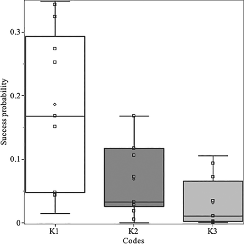
Experiments have been programmed in ProjectQ,¹⁵ and carried out on a simulator, using exact energy estimation (through the wavefunction) and classical optimizer L-BFGS-B.¹⁶ In a first experiment, we have run 100 instances of level-1 QAOA for codes $K_{1}, K_{2}, K_{3}$ , computing the exact success probability of finding a vector e with prescribed syndrome, and Hamming weight upper bounded by w, that is, of solving the SDP. Table 2 shows the average, maximum, minimum, and SD of such probabilities. Also, a boxplot based on the experiments carried out for codes $K_{1}, K_{2}, K_{3}$ (level-1 QAOA) can be found on Figure 1.

TABLE 2. Success probability of solving the syndrome decoding problem (100 experiments of level-1 quantum approximate optimization algorithm)

Code	s	w	Average	Max	Min	SD
$K_{1}$	$(10000)$	4	0.186	0.349	0.015	0.120
$K_{2}$	$(11010)$	4	0.068	0.168	0	0.060
$K_{3}$	$(01000)$	4	0.031	0.106	0	0.035

Details are in the caption following the image — **FIGURE 1**
Open in figure viewer PowerPoint

Boxplot of success probabilities for codes $K_{1}, K_{2}, K_{3}$ with level-1 quantum approximate optimization algorithm (100 experiments)

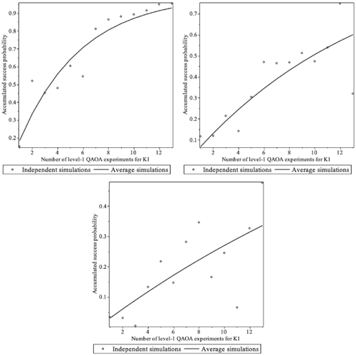
We have used the outcome data to establish accumulated probabilities of success, based both on the average value, and also on the concrete probabilities of the experiments $# 1$ to $# 91$ , to simulate an increasing number ( $1, 2, 3, \dots, 13$ ) of independent experiments. Figure 2 contains the results. As we can see, the success probability decreases with the length n of the code (the rest of the parameters is the same: $k = ⌈ \frac{n}{2} ⌉$ , $w = 4$ , $\max d_{ν} = 2$ ). This is somehow expected, since the number of qubits required by the QAOA is exactly such a length.

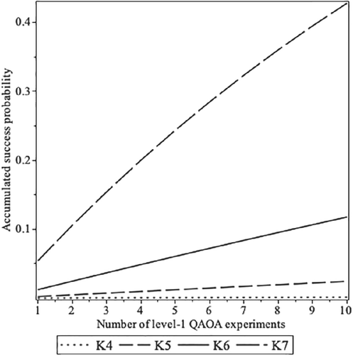
The same experiment was run with 10 instances of level-1 QAOA for codes $K_{4}, K_{5}, K_{6}, K_{7}$ . Table 3 shows the average, maximum, minimum, and SD of the accumulated success probabilities, whereas Figure 3 shows the accumulated success probability based on the average probability obtained in the simulations. Again, we can observe the tendency to obtain smaller success probability with random codes of higher length (here $n = 20$ , for $K_{4}$ ). On the other hand, it has to be noticed that two out of the three Goppa codes ( $K_{6}, K_{7}$ ) have significantly higher success probabilities than the random code ( $K_{4}$ ). This might suggest that these two codes have an inner structure that favors the QAOA. It might be possible that the higher dimension of the Goppa codes have also an effect in the algorithm. However, the success probability of the third Goppa code ( $K_{5}$ ) apparently goes against this conclusion.

TABLE 3. Success probability of solving the syndrome decoding problem (10 experiments of level-1 quantum approximate optimization algorithm). Probabilities are to be multiplied by a factor of

1 0^{- 4}

Code	s	w	Average	Max	Min	SD
$K_{4}$	$(1101110101)$	5	1.513	5.052	0	1.972
$K_{5}$	$(1111)$	1	24.767	84.115	0.002	37.818
$K_{6}$	$(0001)$	1	124.551	351.927	0	128.060
$K_{7}$	$(0000)$	1	543.092	2713.267	0.025	1085.087

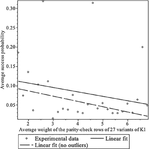
A third experiment was run with the 27 variants of code $K_{1}$ introduced above. In all cases, 100 level-1 QAOA simulations where carried out. The average, maximum, minimum, and SD of the success probabilities are collected in Table 4. Figure 4 shows how the success probability changes when increasing the average number of ones per row of the parity-check matrix H. The data show a certain tendency toward higher success probabilities among those variants with smaller number of ones. This might suggest the cryptographic use of codes presented through parity-check matrices with as many ones as possible.

TABLE 4. Success probability of solving the syndrome decoding problem for the 27 variants of the code

K_{1}

(100 experiments of level-1 quantum approximate optimization algorithm)

Variant	s	$\overline{d_{ν}}$	Average	Max	Min	SD
1	$(00001)$	$\frac{8}{5}$	0.186	0.349	0.016	0.112
2	(00001)	$\frac{9}{5}$	0.074	0.242	0	0.087
3	(10001)	2	0.135	0.244	0.027	0.063
4	(00001)	$\frac{11}{5}$	0.036	0.219	0	0.057
5	(00001)	$\frac{12}{5}$	0.103	0.246	0.007	0.080
6	(00001)	$\frac{13}{5}$	0.318	0.958	0.008	0.333
7	(10001)	$\frac{14}{5}$	0.111	0.216	0.007	0.066
8	(11001)	3	0.015	0.094	0	0.018
9	(11001)	$\frac{16}{5}$	0.032	0.192	0	0.038
10	(01001)	$\frac{17}{5}$	0.040	0.168	0	0.045
11	(11001)	$\frac{18}{5}$	0.038	0.179	0	0.049
12	(10001)	$\frac{19}{5}$	0.076	0.215	0.010	0.070
13	(11001)	4	0.032	0.164	0	0.050
14	(11001)	$\frac{21}{5}$	0.029	0.149	0	0.033
15	(01001)	$\frac{22}{5}$	0.051	0.164	0.007	0.049
16	(11001)	$\frac{23}{5}$	0.314	0.960	0.004	0.365
17	(11101)	$\frac{24}{5}$	0.041	0.142	0	0.044
18	(11101)	5	0.055	0.133	0	0.044
19	(11101)	$\frac{26}{5}$	0.039	0.129	0.001	0.038
20	(11111)	$\frac{27}{5}$	0.029	0.151	0	0.033
21	(11111)	$\frac{28}{5}$	0.029	0.138	0.001	0.028
22	(10100)	$\frac{29}{5}$	0.033	0.131	0.005	0.024
23	(10110)	6	0.053	0.125	0.003	0.033
24	(01110)	$\frac{31}{5}$	0.030	0.101	0	0.0202
25	(11100)	$\frac{32}{5}$	0.064	0.125	0.024	0.030
26	(01110)	$\frac{33}{5}$	0.200	0.961	0.008	0.317
27	(01111)	$\frac{34}{5}$	0.049	0.153	0.002	0.036

We have tested higher level QAOA for the codes $K_{1}, K_{2}, K_{3}$ (10 independent experiments each). The average, maximum, minimum, and SD of the success probabilities are collected in Tables 5–7. Figure 5 shows the success probability change when the level p is increased from 1 to 5. As expected, the higher the depth, the better results that the QAOA yields. Since the Hamiltonian cost of those codes is an Ising model ( $\max d_{ν} = 2$ ), we have tested 5000 experiments in the DWave Quantum Annealer.¹⁷ The same figure plots the average success probability of these experiments. It should be noticed that the QAOA is a remarkable alternative to the adiabatic computation performed by the quantum annealer (at least for the codes studied, with lengths $n = 10, 11, 12$ ).

TABLE 5. Success probabilities for code

K_{1}

with quantum approximate optimization algorithm of levels 1–5

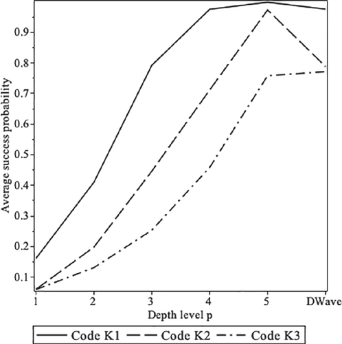
p	Average	Maximum	Minimum	SD
1	0.161	0.349	0.015	0.137
2	0.410	0.560	0.310	0.075
3	0.793	0.959	0.573	0.105
4	0.976	0.999	0.925	0.025
5	0.999	0.999	0.995	0.001

TABLE 6. Success probabilities for code

K_{2}

with quantum approximate optimization algorithm of levels 1–5

p	Average	Maximum	Minimum	SD
1	0.060	0.168	0	0.062
2	0.198	0.470	0.037	0.103
3	0.446	0.871	0.0560	0.255
4	0.712	0.970	0.173	0.225
5	0.974	1	0.932	0.025

TABLE 7. Success probabilities for code

K_{3}

with quantum approximate optimization algorithm of levels 1-5

p	Average	Maximum	Minimum	SD
1	0.059	0.094	0.002	0.038
2	0.131	0.441	0.001	0.123
3	0.253	0.776	0.001	0.200
4	0.459	0.683	0.222	0.160
5	0.759	0.999	0.337	0.188

4 CONCLUSIONS AND FUTURE WORK

In this paper, we have applied the QAOA to an $N P$ -complete problem from Coding Theory upon which relies the security of several postquantum cryptographic schemes. We have modeled the problem in suitable terms to apply the hybrid classical-quantum algorithm and we have experimentally checked its correctness. We have made some experiments from codes obtained from the site.² Among them, the (accumulated) success probabilities for seven different codes (including 3 binary Goppa codes), for 27 variants of the same random code for QAOA of depth level 1. We have also experimented with higher level QAOA ( $p = 1$ –5) for the same code. The experiments suggests that random codes with a higher length, and presented by parity-check matrices of high density, are more resistant to the QAOA algorithm, at least for small depths and on simulations. Unfortunately, because of the current state of quantum technology, we have been able to test any Quasi-Cyclic code of those contained in.² Experimenting with codes of higher length, or the modification of the Hamiltonian to cope with the challenge of the Large weight syndrome decoding problem² is future work.

ACKNOWLEDGMENTS

This work was supported in part by the MINECO under Grant MTM-2017-83506-C2-2-P and Grant MINECO-16-TEC2015-67387-C4-3-R, and in part by the MICINN under Grant RTI2018-098085-B-C44, Grant FC-GRUPIN-IDI/2018/000193, and under Grant FC-GRUPIN-IDI/2018/000226.

Biographies

Markel Epelde received the B.S. and M.S. degrees in mathematics from the University of the Basque Country, Spain, in 2015, and 2016, respectively. Currently, he is a Ph.D. student in the University of the Basque Country.
Elías F. Combarro received the B.S. degree in mathematics, the M.S. degree in computer science, and the Ph.D. degree in mathematics from the University of Oviedo, Oviedo, Spain, in 1997, 2001, and 2002, respectively, where he is currently an Associate Professor. He has authored more than 30 research papers in topics such as computability theory, the theory of fuzzy measures, and the computational classification of semifields and text categorization. His current research interest includes quantum computing.
Ignacio F. Rúa received the B.S., M.S., and Ph.D. degrees in mathematics from the University of Oviedo, Oviedo, Spain, in 1999, 2001, and 2004, respectively, where he is currently an Associate Professor. From 2004 to 2007, he was a Research Fellow of the Spanish Juan de la Cierva Program with the Universidad de Cantabria. He has coauthored 30 research papers on nonassociative finite rings and their applications in coding theory and cryptography. His current research interests include computer algebra and quantum computing.

REFERENCES

1Huffman WC, Brualdi RA, Pless VS. Handbook of Coding Theory. Elsevier Science Inc.; 1998.
Google Scholar
2 Decoding challenge; July 2021. https://decodingchallenge.org
Google Scholar
3 Post-quantum cryptography standardization process; July 2021. https://csrc.nist.gov/Projects/post-quantum-cryptography
Google Scholar
4Berlekamp E, McEliece R, Van Tilborg H. On the inherent intractability of certain coding problems. IEEE Trans Inf Theory. 1978; 24(3): 384-386. doi:10.1109/TIT.1978.1055873
10.1109/TIT.1978.1055873
Web of Science® Google Scholar
5Stern J. A new paradigm for public key identification; 1996:13-21. doi: 10.1109/18.556672
Google Scholar
6Aaronson S. The limits of quantum computers. In: V Diekert, MV Volkov, A Voronkov, eds. Computer Science - Theory and Applications, Second International Symposium on Computer Science in Russia, CSR 2007, Ekaterinburg, Russia, September 3-7, 2007, Proceedings, Lecture Notes in Computer Science. Vol 4649. Springer; 2007: 4.
10.1007/978-3-540-74510-5_2
Google Scholar
7Farhi E, Goldstone J, Gutmann S. A quantum approximate optimization algorithm; 2014. arXiv:1412.6062.
Google Scholar
8Matsumine T, Koike-Akino T, Wang Y. Channel decoding with quantum approximate optimization algorithm; 2019.
Google Scholar
9Farhi E, Goldstone J, Gutmann S, Sipser M. Quantum computation by adiabatic evolution; 2000. arXiv:quant-ph/0001106v1.
Google Scholar
10Aharonov D., Dam W., Kempe J., Landau Z., Loyd S., Regev O.. Adiabatic quantum computation is equivalent to standard quantum computation; Vol. 45, 2004:42-51.
Google Scholar
11Wang H, Wu L-A. Ultrafast adiabatic quantum algorithm for the NP-complete exact cover problem. Sci Rep. 2016; 6:22307 EP.
10.1038/srep22307
Web of Science® Google Scholar
12Born M, Fock V. Beweis des Adiabatensatzes. Zeitschrift für Physik. 1928; 51(3-4): 165-180.
10.1007/BF01343193
CAS Google Scholar
13McGeoch CC. Adiabatic Quantum Computation and Quantum Annealing. Synthesis Lectures on Quantum Computing. Morgan&Claypool Publishers; 2014.
10.1007/978-3-031-02518-1
Google Scholar
14Suzuki M. Generalized Trotter's formula and systematic approximants of exponential operators and inner derivations with applications to many-body problems. Commun Math Phys. 1976; 51(2): 183-190. doi:10.1007/BF01609348
10.1007/BF01609348
Web of Science® Google Scholar
15 ProjectQ software; July 2021. http://projectq.ch/
Google Scholar
16Byrd RH, Lu P, Nocedal J, Zhu C. A limited memory algorithm for bound constrained optimization. SIAM J Sci Comput. 1995; 16(5): 1190-1208. doi:10.1137/0916069
10.1137/0916069
ADS Web of Science® Google Scholar
17 D-Wave leap; July 2021. https://www.dwavesys.com/take-leap
Google Scholar

All articles

Quantum approximate optimization of the coset leader problem for binary linear codes

Abstract

1 INTRODUCTION

2 QAOA FOR CLP

3 EXPERIMENTAL RESULTS ON QAOA FOR CLP

4 CONCLUSIONS AND FUTURE WORK

ACKNOWLEDGMENTS

Biographies

REFERENCES

Figures

References

Information

About Wiley Online Library

Help & Support

Opportunities

Connect with Wiley

Quantum approximate optimization of the coset leader problem for binary linear codes

Abstract

1 INTRODUCTION

2 QAOA FOR CLP

3 EXPERIMENTAL RESULTS ON QAOA FOR CLP

4 CONCLUSIONS AND FUTURE WORK

ACKNOWLEDGMENTS

Biographies

REFERENCES

Figures

References

Related

Information