This study aims at constructing a robust numerical scheme for solving singularly perturbed parabolic delay differential equations arising in the modeling of neuronal variability. Taylor's series expansion is applied to approximate the shift terms. The obtained result is approximated by using the implicit Euler method in the temporal discretization on a uniform step size with the hybrid numerical scheme consisting of the midpoint upwind method in the outer layer region and the cubic spline in tension method in the inner layer region on a piecewise uniform Shishkin mesh in the spatial discretization. The constructed scheme is shown to be an $ε$ -uniformly convergent accuracy of order $O (Λ t + N^{- 2} \ln^{3} N)$ . Two model examples are given to testify the theoretical findings.

1 INTRODUCTION

The motivation for the considered problem in this article relies on the mathematical model given by Stein,¹ about the time evolution trajectories of the membrane potential in terms of singularly perturbed parabolic delay differential equations (SPPDDEs) as:

\frac{\partial u}{\partial t} + \frac{σ^{2}}{2} \frac{\partial^{2} u}{\partial x^{2}} + (ζ_{D} - \frac{x}{θ}) \frac{\partial u}{\partial x} + λ_{s} u (x + a_{s}, t) + ω_{s} u (x + i_{s}, t) - (λ_{s} + ω_{s}) u (x, t) = 0,

()

where

σ

and

ζ_{D}

are diffusion moments of Wiener process characterizing the influence of dendritic synapses on the cell excitability. The membrane potential decays exponentially to the resting level with a membrane time constant

θ

. The first derivative term is obtained because of the exponential decay between two consecutive jumps caused by the input processes. The reaction terms correspond to the superposition of excitatory and inhibitory inputs, and we can assume that they are Poissonian.² This model makes available time evolution of the trajectories of the membrane potential. The excitatory input contributes to the membrane potential by an amplitude

a_{s}

with intensity

λ_{s}

and similarly, the inhibitory input contributes by an amplitude

i_{s}

with intensity

ω_{s}

. Because of the problematical structure of the model (1), one can hardly obtain its exact solution. Therefore, to capture the behavior of this model, it is very important to devise efficient numerical methods that provide more accurate approximate solutions to the problem.

Since the past decade, some scholars have been developing robust numerical methods for the SPPDDE with shift parameter(s) and analyzing the effects of the shift parameters on the solution profile. The authors^3-12 have developed different numerical methods based on fitting techniques (adaptive layer and fitted operator) for solving the SPPDDE with shift(s) in the space variable and elucidated the effect of the singular perturbation and shift parameter(s) on the solution profile. The authors^13-16 have also suggested various robust numerical schemes for SPPDDE with time delay. Recently, the authors^17-19 have presented higher-order a parameter uniform computational methods for singularly perturbed two-parameter parabolic convection–diffusion problems using a fitted operator. However, numerical methods to solve the SPPDDE with mixed small shifts in the spatial variable having an $ε$ -uniform convergence for the past decades are still few. The main contribution of this study is to construct and analyze a robust numerical scheme to solve the families of the problem under consideration that arises in the modeling of neuronal variability. The formulation of the method and its corresponding error analysis are treated in the subsequent sections.

Standard supremum norm is denoted by ${‖\cdot‖}_{\infty}$ and is defined by ${‖ϑ‖}_{\infty} = \sup_{(x, t) \in D} |ϑ (x, t)|$ , for a function $ϑ$ defined on some domain D.

2 CONTINUOUS PROBLEM

Consider the following governing problem on the domain

D = Ω_{x} \times Ω_{t} = (0, 1) \times (0, T]

\{\begin{array}{ll} \frac{\partial u (x, t)}{\partial t} - ε^{2} \frac{\partial^{2} u (x, t)}{\partial x^{2}} + A (x) \frac{\partial u (x, t)}{\partial x} + B (x) u (x - δ, t) + F (x) u (x, t) + G (x) u (x + η, t) = ϑ (x, t), (x, t) \in D, \\ u (x, 0) = u_{0} (x), x \in D_{0} = {{(x, 0) : x \in \overline{Ω}}_{x}}, \\ u (x, t) = Υ_{1} (x, t), \forall (x, t) \in D_{L} = \{(x, t) : - δ \leq x \leq 0, t \in (0, T]\}, \\ u (x, t) = Υ_{2} (x, t), \forall (x, t) \in D_{R} = \{(x, t) : 1 \leq x \leq 1 + η, t \in (0, T]\}, \end{array}

()

where

0 < ε ≪ 1

is a singular perturbation parameter and delay parameter

δ

and advance parameter

η

are of

o (ε)

. The functions

A (x), B (x), F (x), G (x)

ϑ (x, t), Υ_{1} (x, t), Υ_{2} (x, t)

and

u_{0} (x)

are considered to be sufficiently smooth, bounded and independent of

ε

. It is also considered that

B (x) + F (x) + G (x) \geq γ > 0, \forall x \in {\overline{Ω}}_{x}

for some positive constant

γ

Following the work in Reference 20, we approximate the terms with small shifts (

δ, η < ε

) using Taylor's series expansion as

u (x - δ, t) = u (x, t) - δ \frac{\partial u (x, t)}{\partial x} + O (δ^{2}),

()

u (x + η, t) = u (x, t) + η \frac{\partial u (x, t)}{\partial x} + O (η^{2}) .

()

Now inserting Equations (3) and (4) into Equation (2) yields

\{\begin{array}{l} L_{ε} \overline{u} (x, t) = ϑ (x, t), \\ \overline{u} (x, 0) = u_{0} (x), x \in {\overline{Ω}}_{x}, \\ \overline{u} (0, t) = Υ_{1} (0, t), t \in {\overline{Ω}}_{t}, \\ \overline{u} (1, t) = Υ_{2} (1, t), t \in {\overline{Ω}}_{t}, \end{array}

()

where

L_{ε} \overline{u} (x, t) = \frac{\partial \overline{u} (x, t)}{\partial t} - ε^{2} \frac{\partial^{2} \overline{u} (x, t)}{\partial x^{2}} + μ (x) \frac{\partial \overline{u} (x, t)}{\partial x} + ν (x) \overline{u} (x, t)

μ (x) = A (x) - δ B (x) + η G (x)

, and

ν (x) = B (x) + F (x) + G (x)

. Since

μ (x) \geq \hat{μ} > 0

and

ν (x) \geq \hat{ν} > 0

for some constants

\hat{μ}

and

\hat{ν}

the solution of Equation (5) exhibits boundary layer near

x = 1

. For small

δ, η

, Equations (2) and (5) have almost equal approximate solution. Here, it is worthwhile to mention that the transition from the Equation (2) to the asymptotically equivalent Equation (5) using the Taylor's series approximation procedure is admitted because of the arguments namely the delay (

δ

) and advance (

η

) are assumed to be of small order of

ε

(i.e.,

δ, η < ε

). For more details on the validity of this transition, one may refer References 21-23.

To elude conflict between boundary and initial condition, we assume the compatibility conditions on the corner of the domain

(0, 0)

and

(0, 1)

as²⁴

\{\begin{array}{ll} {\overline{u}}_{0} (0) = Υ_{1} (0, 0), \\ {\overline{u}}_{0} (1) = Υ_{2} (1, 0), \end{array}

()

and

\{\begin{array}{ll} \frac{\partial Υ_{1} (0, 0)}{\partial t} - ε^{2} \frac{\partial^{2} {\overline{u}}_{0} (0)}{\partial x^{2}} + μ (0) \frac{\partial {\overline{u}}_{0} (0)}{\partial x} + ν (0) {\overline{u}}_{0} (0) = ϑ (0, 0), \\ \frac{\partial Υ_{2} (1, 0)}{\partial t} - ε^{2} \frac{\partial^{2} {\overline{u}}_{0} (1)}{\partial x^{2}} + μ (1) \frac{\partial {\overline{u}}_{0} (1)}{\partial x} + ν (1) {\overline{u}}_{0} (1) = ϑ (1, 0) . \end{array}

()

Lemma 1.(Maximum principle). Let $Ξ (x, t) \in C^{2, 1} (\overline{D})$ . If $Ξ (x, t) \geq 0, \forall (x, t) \in \partial D$ ( $\partial D = \overline{D} - D$ ) and $L_{ε} Ξ (x, t) \geq 0, \forall (x, t) \in D$ , then $Ξ (x, t) \geq 0, \forall (x, t) \in \overline{D}$ .

Proof.See Reference 6.

Lemma 2. (Stability estimate)Let $\overline{u} (x, t)$ be the solution of Equation (5), then we have the estimation

{‖\overline{u}‖}_{\overline{D}} \leq {‖\overline{u}‖}_{\partial D} + \frac{{‖ϑ‖}_{\overline{D}}}{\hat{ν}} .

()

Proof.Defining the barrier functions $Ξ^{\pm} (x, t)$ as

Ξ^{\pm} (x, t) = {‖\overline{u}‖}_{\partial D} + \frac{{‖ϑ‖}_{\overline{D}}}{\overline{ν}} \pm \overline{u} (x, t), (x, t) \in \overline{D} .

On applying the maximum principle, we obtain the required bound.

3 DESCRIPTION OF THE NUMERICAL SCHEME

To formulate the numerical scheme, we first discretize the temporal variable using the implicit Euler method on a uniform mesh.

3.1 Temporal discretization

We divide the time domain

[0, T]

into M equidistant with time step size

Λ t

such that

D_{Λ t}^{M} = \{(x, t_{j + 1}) : x \in Ω_{x}, t_{j + 1} = j Λ t, Λ t = \frac{T}{M}, \forall 1 \leq j \leq M - 1\} .

Applying the implicit Euler scheme on t yields

\{\begin{array}{ll} (I + Λ t L_{ε}^{M}) U^{j + 1} (x) = Λ t ϑ^{j + 1} (x) + U^{j} (x), \\ U (x, 0) = U_{0} (x), x \in {\overline{Ω}}_{x}, \\ U^{j + 1} (0) = Υ_{1}^{j + 1} (0), t \in {\overline{Ω}}_{t}, \\ U^{j + 1} (1) = Υ_{2}^{j + 1} (1), t \in {\overline{Ω}}_{t}, \end{array}

()

where

L_{ε}^{M} U^{j + 1} (x) = - ε^{2} \frac{d^{2} U^{j + 1} (x)}{d x^{2}} + μ (x) \frac{d U^{j + 1} (x)}{d x} + ν (x) U^{j + 1} (x) .

Lemma 3. (Discrete maximum principle)Let $Ξ^{j + 1} (x) \in C^{2} ({\overline{Ω}}_{x})$ . If $Ξ^{j + 1} (0) \geq 0,$ $Ξ^{j + 1} (1) \geq 0,$ and $(I + Λ t L_{ε}^{M}) Ξ^{j + 1} (x) \geq 0, \forall x \in Ω_{x}$ , then $Ξ^{j + 1} (x) \geq 0, \forall x \in {\overline{Ω}}_{x}$ .

Proof.See Reference 11.

Lemma 4.Suppose $|\frac{\partial^{k} \overline{u} (x, t)}{\partial t^{k}}| \leq C, \forall (x, t) \in (\overline{D}), k = 0, 1, 2$ , then the local error estimate $e_{j + 1} = \overline{u} (x, t_{j + 1}) - U (x, t_{j + 1})$ in the temporal discretization at $(j + 1)$ th time level satisfies

{‖e_{j + 1}‖}_{\infty} \leq C {(Λ t)}^{2} .

Proof.The detailed proof of this lemma is given in Reference 5.

Lemma 5.The global error estimate $E_{j}$ in the temporal direction of Equation (9) satisfies

{‖E_{j}‖}_{\infty} \leq C (Λ t), \forall j \leq T / Λ t .

Proof.From Lemma 4, we have

\begin{align} {‖E_{j}‖}_{\infty} & = {‖\sum_{k = 1}^{j} e_{k}‖}_{\infty} \leq {‖e_{1}‖}_{\infty} + {‖e_{2}‖}_{\infty} + {‖e_{3}‖}_{\infty} + \dots + {‖e_{j}‖}_{\infty}, \\ \leq c_{1} j {(Λ t)}^{2}, by Lemma 4, \\ \leq c_{1} (j Λ t) Λ t, \\ \leq c_{1} T (Λ t), (j Λ t \leq T), \\ \leq C (Λ t), \end{align}

()

where C is a positive constant independent of

ε

and

Λ t

. Therefore, the time semidiscretization process is uniformly convergent of first order.

Theorem 1.The semidiscretize solution $U^{j + 1} (x)$ and its derivatives satisfy the following bounds:

|\frac{d^{k} U^{j + 1} (x)}{d x^{k}}| \leq C (1 + {(ε^{2})}^{- k} \exp (- \hat{μ} \frac{(1 - x)}{ε^{2}})), for 0 \leq k \leq 4 .

Proof.See Reference 5.

To get the strong derivatives bound of the solution of Equation (9), we decompose the solution into the regular and singular parts as

U^{j + 1} (x) = V^{j + 1} (x) + W^{j + 1} (x),

where the regular part

V^{j + 1} (x)

is the solution of the nonhomogeneous problem

\{\begin{array}{ll} (I + Λ t L_{ε}^{M}) V^{j + 1} (x) = Λ t ϑ^{j + 1} (x) + + V^{j + 1} (x), \forall (x, t_{j + 1}) \in D^{M}, \\ V^{j + 1} (0) = U^{j + 1} (0), \forall t_{j + 1} \in Ω_{t}^{M}, \\ V^{j + 1} (1) = U^{j + 1} (1), \forall t_{j + 1} \in Ω_{t}^{M}, \end{array}

and the singular part

W^{j + 1} (x)

of the homogeneous problem

\{\begin{array}{ll} (I + Λ t L_{ε}^{M}) W^{j + 1} (x) = 0, \forall (x, t_{j + 1}) \in D^{M}, \\ W^{j + 1} (0) = 0, \forall t_{j + 1} \in Ω_{t}^{M}, \\ W^{j + 1} (1) = V^{j + 1} (1) - U^{j + 1} (1), \forall t_{j + 1} \in Ω_{t}^{M} . \end{array}

Lemma 6. ([6])The regular and singular components of $U^{j + 1} (x)$ satisfies the following bounds

|\frac{d^{k} V^{j + 1} (x)}{d x^{k}}| \leq C (1 + {(ε^{2})}^{2 - k}),

|\frac{d^{k} W^{j + 1} (x)}{d x^{k}}| \leq C ({(ε^{2})}^{- k} \exp (- \hat{μ} \frac{(1 - x)}{ε^{2}})), for 0 \leq k \leq 3 .

3.2 Spatial discretization

Mesh selection strategy

Since the boundary value problem (9) exhibits a strong boundary layer at

x = 1

, we choose a piecewise-uniform Shishkin mesh and divide the domain

{\overline{Ω}}_{x} = [0, 1]

into two subintervals, namely,

[0, 1 - τ]

, and

[1 - τ, 1]

. Here, the transition parameter

τ

is defined as:

τ = \min (\frac{1}{2}, τ_{0} ε^{2} \ln (N)), τ_{0} \geq \frac{1}{\hat{μ}} .

The mesh

{\overline{Ω}}_{x}

is given by:

x_{i} = \{\begin{array}{ll} i h_{i}, & for i = 0, 1, 2, \dots, N / 2, \\ 1 - τ + (i - \frac{N}{2}) h_{i}, & for i = N / 2 + 1, N / 2 + 2, \dots, N, \end{array}

where

h_{i} = x_{i} - x_{i - 1} = \{\begin{array}{ll} \frac{2 (1 - τ)}{N}, & for i = 1, 2, \dots, N / 2, \\ \frac{2 τ}{N}, & for i = N / 2 + 1, N / 2 + 2, \dots, N . \end{array}

3.2.1 Hybrid numerical scheme

In this subsection, we approximate Equation (9) by using the hybrid numerical scheme which is based on the midpoint upwind difference method in the outside layer region and cubic spline in tension method in the inside layer region.

Midpoint upwind method

Let us rewrite equation (9) as:

\{\begin{array}{ll} L_{ε}^{M} U^{j + 1} (x) = g^{j + 1} (x), \\ U^{0} (x) = u_{0} (x), x \in {\overline{Ω}}_{x}, \\ U^{j + 1} {(0)}^{=} Υ_{1}^{j + 1} {(0)}^{}, t \in {\overline{Ω}}_{t}, \\ U^{j + 1} (1) = Υ_{2}^{j + 1} (1), t \in {\overline{Ω}}_{t}, \end{array}

()

where

\begin{align} L_{ε}^{M} U_{i}^{j + 1} & = - ε^{2} \frac{d^{2} U^{j + 1} (x)}{d x^{2}} + μ (x) \frac{d U^{j + 1} (x)}{d x} + ϱ (x) U^{j + 1} (x), ϱ (x) = ν (x) + \frac{1}{Λ t}, \\ g^{j + 1} (x) & = ϑ^{j + 1} (x) + \frac{U^{j} (x)}{Λ t} . \end{align}

Then, the midpoint upwind method for Equation (9) takes the form:

L_{m u}^{N, M} U_{i}^{j + 1} = \{\begin{array}{ll} - ε^{2} D_{x}^{+} D_{x}^{-} U_{i}^{j + 1} + μ_{i - 1 / 2} D_{x}^{-} U_{i}^{j + 1} + ϱ_{i - 1 / 2} U_{i - 1 / 2}^{j + 1} = g_{i - 1 / 2}^{j + 1}, \\ U^{j + 1} (0) = Υ_{1}^{j + 1} (0), t_{j + 1} \in {\overline{Ω}}_{t}, \\ U^{j + 1} (1) = Υ_{2}^{j + 1} (1), t_{j + 1} \in {\overline{Ω}}_{t}, \end{array}

()

where

L_{m u}^{N, M}

is the midpoint upwind finite difference operator,

D_{x}^{-} U_{i}^{j + 1} = \frac{U_{i}^{j + 1} - U_{i - 1}^{j + 1}}{h_{i}},

$D_{x}^{+} D_{x}^{-} U_{i, j + 1} = \frac{2}{h_{i} + h_{i - 1}} (\frac{U_{i + 1}^{j + 1} - U_{i}^{j + 1}}{h_{i}} - \frac{U_{i}^{j + 1} - U_{i - 1}^{j + 1}}{h_{i - 1}}),$ $μ_{i - 1 / 2} = (\frac{μ_{i} + μ_{i - 1}}{2})$ , $ϱ_{i - 1 / 2} = (\frac{ϱ_{i} + ϱ_{i - 1}}{2})$ and $g_{i - 1 / 2}^{j + 1} = (\frac{g_{i}^{j + 1} + g_{i - 1}^{j + 1}}{2})$ .

The resulting scheme gives the following system of equations:

L_{m u}^{N, M} U_{i}^{j + 1} = s_{i}^{-} U_{i - 1}^{j + 1} + s_{i}^{0} U_{i}^{j + 1} + s_{i}^{+} U_{i + 1}^{j + 1} = P_{i}^{j + 1}, i = 1, \dots, N - 1, j = 0, 1, 2, \dots M - 1,

()

where

\begin{align} s_{i}^{-} & = \frac{- 2 ε^{2}}{h_{i - 1} (h_{i} + h_{i - 1})} - \frac{μ_{i - 1 / 2}}{h_{i}} + \frac{ϱ_{i - 1 / 2}}{2}, \\ s_{i}^{0} & = \frac{2 ε^{2}}{h_{i} h_{i - 1}} + \frac{μ_{i - 1 / 2}}{h_{i}} + \frac{ϱ_{i - 1 / 2}}{2}, \\ s_{i}^{+} & = \frac{- 2 ε^{2}}{h_{i} (h_{i} + h_{i - 1})}, \\ P_{i}^{j + 1} & = g_{i - 1 / 2}^{j + 1} . \end{align}

Cubic spline in tension method

Now, we approximate the inside layer region of the resulting spatial equation (11) by applying the cubic spline in tension method as described below.

A function

S^{j + 1} (x, ρ) \in C^{2} [0, 1]

which interpolates

U^{j + 1} (x_{i})

i = 0 (1) N

depends on a parameter

ρ > 0

reduces to cubic spline in

[0, 1]

ρ \to 0

is termed as parametric cubic spline function. The relation

S^{j + 1} (x, ρ) = S^{j + 1} (x)

satisfying in

[x_{i}, x_{i + 1}]

\begin{array}{ll} \frac{d^{2} S^{j + 1} (x)}{d x^{2}} + ρ S^{j + 1} (x) = [\frac{d^{2} S^{j + 1} (x_{i})}{d x^{2}} + ρ S^{j + 1} (x_{i})] (\frac{x_{i + 1} - x}{h}) + [\frac{d^{2} S^{j + 1} (x_{i + 1})}{d x^{2}} + ρ S^{j + 1} (x_{i + 1})] (\frac{x - x_{i}}{h}), \end{array}

()

where

S^{j + 1} (x_{i}) = U_{i}^{j + 1}

and

ρ > 0

is known to be cubic spline in tension.

Following Reference 25, we can obtain the following scheme

λ_{1} h_{i} M_{i + 1}^{j + 1} + λ_{2} (h_{i} + h_{i - 1}) M_{i}^{j + 1} + λ_{1} h_{i - 1} M_{i - 1}^{j + 1} = \frac{U_{i + 1}^{j + 1} - U_{i}^{j + 1}}{h_{i}} - \frac{U_{i}^{j + 1} - U_{i - 1}^{j + 1}}{h_{i - 1}}, for i = 1, 2, \dots N - 1,

()

where

λ_{1} = \frac{1}{λ^{2}} (1 - \frac{λ}{\sinh λ}), λ_{2} = \frac{1}{λ^{2}} (λ \coth λ - 1)

λ = h ρ^{1 / 2}

, and

M_{k} = \frac{d^{2} S^{j + 1} (x_{k})}{d x^{2}}, k = i, i \pm 1

. For the choice of parameters

λ_{1} + λ_{2} = 1 / 2

, Equation (15) is consistent and suitable for solving the given differential equation.

Using Taylor's series approximations for

U^{j + 1} (x_{k}), k = i \pm 1

in the spatial variable, we have:

U^{j + 1} (x_{i - 1}) \approx U^{j + 1} (x_{i}) - h_{i - 1} \frac{d U^{j + 1} (x_{i})}{d x} + \frac{h_{i - 1}^{2}}{2} \frac{d^{2} U^{j + 1} (x_{i})}{d x^{2}},

()

U^{j + 1} (x_{i + 1}) \approx U^{j + 1} (x_{i}) + h_{i} \frac{d U^{j + 1} (x_{i})}{d x} + \frac{h_{i}^{2}}{2} \frac{d^{2} U^{j + 1} (x_{i})}{d x^{2}} .

()

Multiplying Equation (16) by

h_{i}^{2} / h_{i - 1}^{2}

and then subtracting the resulting equations from Equation (17), we have:

\frac{d U^{j + 1} (x_{i})}{d x} \approx \frac{1}{h_{i} h_{i - 1} (h_{i} + h_{i - 1})} (- h_{i}^{2} U^{j + 1} (x_{i - 1}) + (h_{i}^{2} - h_{i - 1}^{2}) U^{j + 1} (x_{i}) + h_{i - 1}^{2} U^{j + 1} (x_{i + 1})) .

()

Similarly, multiplying Equation (16) by

h_{i} / h_{i - 1}

and then adding the resulting equations to Equation (17), we get:

\frac{d^{2} U^{j + 1} (x_{i})}{d x^{2}} \approx \frac{2}{h_{i} h_{i - 1} (h_{i} + h_{i - 1})} (h_{i} U^{j + 1} (x_{i - 1}) + (h_{i} + h_{i - 1}) U^{j + 1} (x_{i}) + h_{i - 1} U^{j + 1} (x_{i + 1})) .

()

Inserting Equations (18) and (19) in

\frac{d U^{j + 1} (x_{i + 1})}{d x} \approx \frac{d U^{j + 1} (x_{i})}{d x} + h_{i} \frac{d^{2} U^{j + 1} (x_{i + 1})}{d x^{2}}

and

\frac{d U^{j + 1} (x_{i - 1})}{d x} \approx \frac{d U^{j + 1} (x_{i})}{d x} + h_{i - 1} \frac{d^{2} U^{j + 1} (x_{i + 1})}{d x^{2}}

, we obtain

\begin{align} \frac{d U^{j + 1} (x_{i - 1})}{d x} & \approx \frac{1}{h_{i} h_{i - 1} (h_{i} + h_{i - 1})} (- (h_{i}^{2} + 2 h_{i} h_{i - 1}) U^{j + 1} (x_{i - 1}) + {(h_{i} + h_{i - 1})}^{2} U^{j + 1} (x_{i})) \\ - \frac{1}{h_{i} h_{i - 1} (h_{i} + h_{i - 1})} (h_{i - 1}^{2} U^{j + 1} (x_{i + 1})) . \end{align}

()

\begin{align} \frac{d U^{j + 1} (x_{i + 1})}{d x} & \approx \frac{1}{h_{i} h_{i - 1} (h_{i} + h_{i - 1})} (- h_{i}^{2} U^{j + 1} (x_{i - 1}) - {(h_{i} + h_{i - 1})}^{2} U^{j + 1} (x_{i})) \\ + \frac{1}{h_{i} h_{i - 1} (h_{i} + h_{i - 1})} ((h_{i}^{2} + 2 h_{i} h_{i - 1}) U^{j + 1} (x_{i + 1})) . \end{align}

()

Equation (9) at

x = x_{k}, k = i, i \pm 1

can be written as:

- ε^{2} M_{k} + μ_{k} \frac{d U^{j + 1} (x_{k})}{d x} + ϱ_{k} U^{j + 1} (x_{k}) = g^{j + 1} (x_{k}) .

()

Taking Equations (18) and (21) into Equation (22) and substituting the resulting equation into Equation (15) yields

L_{c s}^{N, M} = r_{i}^{-} U_{i - 1}^{j + 1} + r_{i}^{0} U_{i}^{j + 1} + r_{i}^{+} U_{i + 1}^{j + 1} = z_{i}^{j + 1}, i = 1, \dots, N - 1, j = 0, 1, 2, \dots M - 1,

()

where

L_{c s}^{N}

is the cubic spline in tension operator,

\begin{align} r_{i}^{-} & = - \frac{ε^{2}}{h_{i - 1} (h_{i - 1} + h_{i})} - λ_{1} \frac{μ_{i - 1} (h_{i} + 2 h_{i - 1})}{{(h_{i} + h_{i - 1})}^{2}} - λ_{2} \frac{μ_{i} h_{i}}{h_{i - 1} (h_{i - 1} + h_{i})} \\ + λ_{1} \frac{μ_{i + 1} h_{i}^{2}}{h_{i - 1} {(h_{i} + h_{i - 1})}^{2}} + λ_{1} ϱ_{i - 1} \frac{h_{i - 1}}{(h_{i - 1} + h_{i})}, \\ r_{i}^{0} & = \frac{ε^{2} (h_{i} + h_{i - 1})}{h_{i} h_{h_{i - 1}} (h_{i - 1} + h_{i})} + λ_{1} \frac{μ_{i - 1}}{h_{i}} + λ_{2} \frac{μ_{i} (h_{i} - h_{i - 1})}{h_{i} h_{i - 1}} - λ_{1} \frac{μ_{i + 1}}{h_{i - 1}} + λ_{2} ϱ_{i}, \\ r_{i}^{+} & = - \frac{ε^{2}}{h_{i} (h_{i - 1} + h_{i})} - λ_{1} \frac{μ_{i - 1} h_{i - 1}^{2}}{h_{i} {(h_{i - 1} + h_{i})}^{2}} + λ_{2} \frac{μ_{i} h_{i - 1}}{h_{i} (h_{i - 1} + h_{i})} \\ + λ_{1} \frac{μ_{i + 1} (h_{i - 1} + 2 h_{i})}{{(h_{i} + h_{i - 1})}^{2}} + λ_{1} ϱ_{i + 1} \frac{h_{i}}{(h_{i - 1} + h_{i})}, \\ z_{i}^{j + 1} & = λ_{1} \frac{h_{i - 1}}{(h_{i - 1} + h_{i})} g_{i - 1}^{j + 1} + λ_{2} g_{i}^{j + 1} + λ_{1} \frac{h_{i}}{(h_{i - 1} + h_{i})} g_{i + 1}^{j + 1} . \end{align}

The fully discrete scheme takes the form:

L_{H y d}^{N, M} U_{i}^{j + 1} = \{\begin{array}{lll} L_{m u}^{N, M} U_{i}^{j + 1} = g_{i - 1 / 2}^{j + 1}, & for & i = 1, 2, \dots, N / 2, \\ L_{c s}^{N, M} U_{i}^{j + 1} = g_{i}^{j + 1}, & for & i = N / 2 + 1, N / 2 + 2, \dots, N, \\ U_{0}^{j + 1} = Υ_{1}^{j + 1} (0), & for & j = 0, \dots, M - 1, \\ U_{N}^{j + 1} = Υ_{2}^{j + 1} (1), & for & j = 0, \dots, M - 1, \\ U_{i}^{0} = U^{0} (x_{i}), & for & i = 0, \dots, N . \end{array}

()

Thus, we obtain the system of linear equations as:

ξ_{i}^{-} U_{i - 1}^{j + 1} + ξ_{i}^{0} U_{i}^{j + 1} + ξ_{i}^{+} U_{i + 1}^{j + 1} = Z_{i}^{j + 1}, i = 1, \dots, N - 1, j = 0, 1, \dots M - 1,

()

where

ξ_{i}^{-} = \{\begin{array}{ll} \frac{- 2 ε^{2}}{h_{i} (h_{i} + h_{i + 1})} - \frac{μ_{i - 1 / 2}}{h_{i + 1}} + \frac{ϱ_{i - 1 / 2}}{2}, & for 0 < i \leq N / 2, \\ - \frac{ε^{2}}{h_{i - 1} (h_{i - 1} + h_{i})} - λ_{1} \frac{μ_{i - 1} (h_{i} + 2 h_{i - 1})}{{(h_{i} + h_{i - 1})}^{2}} - λ_{2} \frac{μ_{i} h_{i}}{h_{i - 1} (h_{i - 1} + h_{i})} + λ_{1} \frac{μ_{i + 1} h_{i}^{2}}{h_{i - 1} {(h_{i} + h_{i - 1})}^{2}} \\ + λ_{1} ϱ_{i - 1} \frac{h_{i - 1}}{(h_{i - 1} + h_{i})}, & for N / 2 < i \leq N . \end{array}

ξ_{i}^{0} = \{\begin{array}{ll} \frac{2 ε^{2}}{h_{i} h_{i + 1}} + \frac{μ_{i - 1 / 2}}{h_{i}} + \frac{ϱ_{i - 1 / 2}}{2}, & for 0 < i \leq N / 2, \\ \frac{ε^{2} (h_{i} + h_{i - 1})}{h_{i} h_{h_{i - 1}} (h_{i - 1} + h_{i})} + λ_{1} \frac{μ_{i - 1}}{h_{i}} + λ_{2} \frac{μ_{i} (h_{i} - h_{i - 1})}{h_{i} h_{i - 1}} - λ_{1} \frac{μ_{i + 1}}{h_{i - 1}} + λ_{2} ϱ_{i}, & for N / 2 < i \leq N . \end{array}

ξ_{i}^{+} = \{\begin{array}{ll} \frac{- 2 ε^{2}}{h_{i + 1} (h_{i} + h_{i + 1})}, & for 0 < i \leq N / 2, \\ - \frac{ε^{2}}{h_{i} (h_{i - 1} + h_{i})} - λ_{1} \frac{μ_{i - 1} h_{i - 1}^{2}}{h_{i} {(h_{i - 1} + h_{i})}^{2}} + λ_{2} \frac{μ_{i} h_{i - 1}}{h_{i} (h_{i - 1} + h_{i})} + λ_{1} \frac{μ_{i + 1} (h_{i - 1} + 2 h_{i})}{{(h_{i} + h_{i - 1})}^{2}} \\ + λ_{1} ϱ_{i + 1} \frac{h_{i}}{(h_{i - 1} + h_{i})}, & for N / 2 < i \leq N . \end{array}

Z_{i}^{j + 1} = \{\begin{array}{ll} g_{i - 1 / 2}^{j + 1}, & for 0 < i \leq N / 2, \\ z_{i}^{j + 1}, & for N / 2 < i \leq N . \end{array}

The matrix representation of Equation (25) is

ξ U = Z .

()

Since $|ξ^{0}| \geq |ξ^{-}| + |ξ^{+}|$ , the matrix $ξ$ is diagonally dominant with $ξ^{0} > 0$ , $ξ^{-} \leq 0$ , and $ξ^{+} \leq 0$ and hence nonsingular and $ξ^{- 1} \geq 0$ . This leads to the matrix $ξ$ is M-matrix and the scheme in (26) has a unique solution. Thus, the tridiagonal systems (26) can be solved using standard direct techniques at each time level.

Lemma 7. (Discrete maximum principle)If $Ξ_{0}^{j + 1} \geq 0,$ $Ξ_{1}^{j + 1} \geq 0,$ then $L_{H y d}^{N, M} Ξ_{i}^{j + 1} \geq 0,$ $\forall i = 1, 2, \dots, N - 1$ implies $Ξ_{i}^{j + 1} \geq 0, \forall i = 0, 1, \dots, N$ .

Proof.The proof follows from similar arguments as used in Lemma 3.

Lemma 8. (Uniform stability estimate)The solution $U_{i}^{j + 1}$ of the scheme in (24) satisfies

‖U_{i}^{j + 1}‖ \leq \frac{‖Z‖}{γ} + C \max \{|Υ_{1}^{j + 1} (0)|, |Υ_{2}^{j + 1} (1)|\}, i = 0, 1, \dots N, j = 0, \dots, M - 1,

where

ϱ_{i} \geq γ > 0

Proof.Consider the barrier functions

{(Ξ_{i}^{j + 1})}^{\pm} = \frac{‖Z‖}{γ} + C \max \{|Υ_{1}^{j + 1} (0)|, |Υ_{2}^{j + 1} (1)|\} \pm U_{i}^{j + 1} .

()

On applying Lemma 7, we obtain the required estimate.

4 ERROR ANALYSIS

This section is devoted to

ε

-uniform convergence for the scheme in (25). The truncation error for

i = N / 2 + 1, \dots, N

is given by

\begin{align} T_{i} & = ξ_{i}^{-} U^{j + 1} (x_{i - 1}) + ξ_{i}^{0} U^{j + 1} (x_{i}) + ξ_{i}^{+} U^{j + 1} (x_{i + 1}) - λ_{1} \frac{h_{i - 1}}{(h_{i} + h_{i - 1})} g^{j + 1} (x_{i - 1}) \\ - λ_{2} g^{j + 1} (x_{i}) - λ_{1} \frac{h_{i}}{(h_{i} + h_{i - 1})} g^{j + 1} (x_{i + 1}), i = 1, \dots, N - 1, j = 0, 1, \dots M - 1 . \end{align}

()

Using Equation (9) for

g^{j + 1} (x_{i + 1}), g^{j + 1} (x_{i})

and

g^{j + 1} (x_{i + 1})

in Equation (28), we obtain

\begin{align} T_{i} & = ξ_{i}^{-} U^{j + 1} (x_{i - 1}) + ξ_{i}^{0} U^{j + 1} (x_{i}) + ξ_{i}^{+} U^{j + 1} (x_{i + 1}) \\ - λ_{1} \frac{h_{i - 1}}{(h_{i} + h_{i - 1})} \{- ε^{2} \frac{d^{2} U^{j + 1} (x_{i - 1})}{d x^{2}} + μ (x_{i - 1}) \frac{d U^{j + 1} (x_{i - 1})}{d x} + ϱ (x_{i - 1}) U^{j + 1} (x_{i - 1})\} \\ - λ_{2} \{- ε^{2} \frac{d^{2} U^{j + 1} (x_{i})}{d x^{2}} + μ (x_{i}) \frac{d U^{j + 1} (x_{i})}{d x} + ϱ (x_{i}) U^{j + 1} (x_{i})\} \\ - λ_{1} \frac{h_{i}}{(h_{i} + h_{i - 1})} \{- ε^{2} \frac{d^{2} U^{j + 1} (x_{i + 1})}{d x^{2}} + μ (x_{i + 1}) \frac{d U^{j + 1} (x_{i + 1})}{d x} + ϱ (x_{i + 1}) U^{j + 1} (x_{i + 1})\}, \\ i = 1, \dots, N - 1, j = 0, 1, \dots M - 1 . \end{align}

()

Using Taylor's series approximation for

U^{j + 1} (x_{i - 1})

and

U^{j + 1} (x_{i + 1}), \frac{d U^{j + 1} (x_{i - 1})}{d x}, \frac{d U^{j + 1} (x_{i + 1})}{d x},

\frac{d^{2} U^{j + 1} (x_{i - 1})}{d x^{2}}

, and

\frac{d^{2} U^{j + 1} (x_{i + 1})}{d x^{2}}

in spatial variable and substituting the resulting equation into Equation (29), we get

T_{i} = τ_{1, i} U^{j + 1} (x_{i}) + τ_{2, i} \frac{d U^{j + 1} (x_{i})}{d x} + τ_{3, i} \frac{d^{2} U^{j + 1} (x_{i})}{d x^{2}} + τ_{4, i} \frac{d^{3} U^{j + 1} (x_{i})}{d x^{3}} + τ_{5, i} \frac{d^{4} U^{j + 1} (x_{i})}{d x^{4}} + \dots,

()

where

\begin{align} T_{1, i} & = ξ_{i}^{-} + ξ_{i}^{0} + ξ_{i}^{+} - λ_{1} \frac{h_{i - 1}}{(h_{i} + h_{i - 1})} ϱ_{i - 1} - λ_{2} ϱ_{i} - λ_{1} \frac{h_{i}}{(h_{i} + h_{i - 1})} ϱ_{i + 1}, \\ T_{2, i} & = - h_{i - 1} ξ^{-} + h_{i} ξ^{+} - λ_{1} \frac{h_{i - 1}^{2}}{(h_{i} + h_{i - 1})} ϱ_{i - 1} - λ_{2} μ_{i} - λ_{1} \frac{h_{i}}{(h_{i} + h_{i - 1})} μ_{i + 1} - λ_{1} \frac{h_{i}^{2}}{(h_{i} + h_{i - 1})} ϱ_{i + 1}, \\ T_{3, i} & = - h_{i - 1}^{2} ξ_{i}^{-} + \frac{h_{i}^{2}}{2} ξ_{i}^{+} + ε^{2} λ_{1} \frac{h_{i - 1}}{(h_{i} + h_{i - 1})} + λ_{1} \frac{h_{i + 1}^{2}}{(h_{i} + h_{i - 1})} μ_{i - 1} - λ_{1} \frac{h_{i - 1}^{3}}{2 (h_{i} + h_{i - 1})} ϱ_{i - 1} - λ_{1} ε^{2} \\ - λ_{1} \frac{h_{i}^{2}}{(h_{i} + h_{i - 1})} μ_{i + 1} + ε^{2} λ_{1} \frac{h_{i}}{(h_{i} + h_{i - 1})} - λ_{1} \frac{h_{i}^{3}}{2 (h_{i} + h_{i - 1})} ϱ_{i + 1}, \\ T_{4, i} & = - \frac{h_{i - 1}^{3}}{6} ξ_{i}^{-} + \frac{h_{i}^{3}}{6} ξ_{i}^{+} - ε^{2} λ_{1} \frac{h_{i - 1}^{2}}{(h_{i} + h_{i - 1})} - λ_{1} \frac{h_{i - 1}^{3}}{2 (h_{i} + h_{i - 1})} μ_{i - 1} + λ_{1} \frac{h_{i - 1}^{4}}{6 (h_{i} + h_{i - 1})} ϱ_{i - 1} \\ + ε^{2} λ_{1} \frac{h_{i}^{2}}{(h_{i} + h_{i - 1})} - λ_{1} \frac{h_{i}^{2}}{2 (h_{i} + h_{i - 1})} μ_{i + 1} - λ_{1} \frac{h_{i}^{4}}{6 (h_{i} + h_{i - 1})} ϱ_{i + 1}, \\ T_{5, i} & = \frac{h_{i - 1}^{4}}{24} ξ_{i}^{-} + + \frac{h_{i}^{4}}{24} ξ_{i}^{+} + ε^{2} λ_{1} \frac{h_{i - 1}^{3}}{2 (h_{i} + h_{i - 1})} + λ_{1} \frac{h_{i - 1}^{4}}{6 (h_{i} + h_{i - 1})} μ_{i - 1} - λ_{1} \frac{h_{i - 1}^{5}}{24 (h_{i} + h_{i - 1})} ϱ_{i - 1} \\ + ε^{2} λ_{1} \frac{h_{i}^{3}}{2 (h_{i} + h_{i - 1})} - λ_{1} \frac{h_{i}^{4}}{6 (h_{i} + h_{i - 1})} μ_{i + 1} - λ_{1} \frac{h_{i}^{5}}{24 (h_{i} + h_{i - 1})} ϱ_{i + 1} . \end{align}

From the above expressions, we get

T_{1, i} = T_{2, i} = 0,

()

and using

λ_{1} + λ_{2} = \frac{1}{2}

in the above expressions, we obtain

\{\begin{array}{ll} T_{3, i} = T_{4, i} = 0, \\ T_{5, i} = - ε^{2} (\frac{1}{24} - \frac{λ_{1}}{2}) (\frac{h_{i - 1}^{3} + h_{i}^{3}}{h_{i - 1} + h_{i}}) . \end{array}

()

Substitution of Equations (31) and (32) into Equation (30) yields

T_{i} = - ε^{2} (\frac{1}{24} - \frac{λ_{1}}{2}) (\frac{h_{i - 1}^{3} + h_{i}^{3}}{h_{i - 1} + h_{i}}) \frac{d^{4} U^{j + 1} (x_{i})}{d x^{4}} + O (Λ t + N^{- 3}) .

()

Applying similar procedures, we obtain the truncation error for

i = 1, \dots, N / 2

T_{i} = - ε^{2} (\frac{h_{i - 1}^{3} + h_{i}^{3}}{h_{i - 1} + h_{i}}) \frac{d^{4} U^{j + 1} (x_{i})}{d x^{4}} + O ((Λ t) + N^{- 3}) .

()

Theorem 2.Let $\overline{u} (x, t)$ be the solution of (5) and $U_{i}^{j + 1}$ be the approximation to the solution of (25), then the following error bound holds

\max_{0 \leq i, j \leq N, M} |\overline{u} (x_{i}, t_{j + 1}) - U_{i}^{j + 1}| \leq C (Λ t + N^{- 2} \ln^{3} N) .

Proof.To estimate the error ${‖\overline{u} (x_{i}, t_{j + 1}) - U_{i}^{j + 1}‖}_{\infty}$ , we follow the following two cases:

Case 1: When $τ = 1 / 2$ , the mesh is uniform with $h = 1 / N$ and $K (ε^{2} / \hat{μ}) \ln N \geq 1 / 2$ , which gives $ε^{- 2} \leq C \ln N$ . By using Theorem 1 in Equations (33) and (34), we obtain

|T_{i}| \leq C (Λ t + N^{- 2} \ln^{3} N) .

()

Case 2: When $τ = K (ε^{2} / \hat{μ}) \ln N$ , the mesh is a piecewise uniform with $h = 2 (1 - τ) / N$ in $[0, 1 - τ]$ and $h = 2 τ / N$ in $[1 - τ, 1]$ .

For the case $1 \leq i \leq N / 2$ , the region is regular region, that is, $[0, 1 - τ]$ . From Lemma 6 we have

|\frac{d^{(k)} U_{i}^{j + 1}}{d x^{(k)}}| \leq C .

()

Using Equation (36) into Equation (34) we obtain

|T_{i}| \leq C (Λ t + N^{- 2}) .

()

For the case $N / 2 < i \leq N$ , the region is boundary layer region, that is, $[1 - τ, 1]$ , we have $h = 2 τ / N = 2 K (ε^{2} / \hat{μ}) N^{- 1} \ln N$ , which gives $h / ε^{2} = C N^{- 1} \ln N$ , therefore from Equation (33), we obtain

|T_{i}| \leq C (Λ t + N^{- 2} \ln^{2} N) .

()

On combining Equations (37) and (38), we get

|T_{i}| \leq C (Λ t + N^{- 2} \ln^{2} N) .

()

Again combining Equations (35) and (39), we obtain the required bound

\max_{0 \leq i, j \leq N, M} |\overline{u} (x_{i}, t_{j + 1}) - U_{i}^{j + 1}| \leq C (Λ t + N^{- 2} \ln^{3} N) .

()

5 NUMERICAL EXAMPLES AND RESULTS

Two examples are presented to testify the theoretical findings. As the exact solutions of these examples are not known, so we compute the maximum pointwise error by using the double mesh principle defined in Reference 8 as:

E_{ε, δ, η}^{N, M} = \max_{1 \leq i, j \leq N - 1, M - 1} |U_{i, j}^{N, M} - U_{i, j}^{2 N, 2 M}|,

where

U_{i, j}^{N, M}

are computed numerical solutions obtained on the mesh

D^{N, M} = Ω_{x}^{N} \times Ω_{t}^{M}

, whereas

U_{i, j}^{2 N, 2 M}

are computed numerical solutions on the mesh

D^{2 N, 2 M} = Ω_{x}^{2 N} \times Ω_{t}^{2 M}

with N and M mesh intervals in the spatial and temporal direction, respectively.

For any value of N and M, the

ε

-uniform maximum error

(E^{N, M})

and the

ε

-uniform rate of convergence

(Γ^{N, M})

are calculated using

E^{N, M} = \max_{ε, δ, η} \{E_{ε, δ, η}^{N, M}\} and Γ^{N, M} = \log_{2} (\frac{E^{N, M}}{E^{2 N, 2 M}}), respectively.

Example 1. ([6])We consider the following SPPDDE of the form in (2)

\{\begin{array}{ll} \frac{\partial u}{\partial t} - ε^{2} \frac{\partial^{2} u}{\partial x^{2}} + (2 - x^{2}) \frac{\partial u}{\partial x} + 2 u (x - δ, t) + (x - 3) u (x, t) + u (x + η, t) = 10 t^{2} \exp^{- t} x (1 - x), \\ u_{0} (x) = 0, Υ_{1} (0, t) = Υ_{2} (1, t) = 0, T = 3 . \end{array}

Example 2. ([8])Now we consider the following SPPDDE of the form in (2)

\{\begin{array}{ll} \frac{\partial u}{\partial t} - ε^{2} \frac{\partial^{2} u}{\partial x^{2}} + (2 - x^{2}) \frac{\partial u}{\partial x} + (1 + x) u (x - δ, t) + (x^{2} + 1 + \cos (π x)) u (x, t) + u (x + η, t) = \sin (π x), \\ u_{0} (x) = 0, Υ_{1} (0, t) = Υ_{2} (1, t) = 0, T = 3 . \end{array}

The computed $E_{ε, δ, η}^{N, M}, E^{N, M}$ , and $Γ^{N, M}$ for Examples 1 and 2 are presented in Tables 1–6. As observed in Tables 1–6 the maximum pointwise errors decrease as the step sizes decrease for all values of $ε$ , which confirms the robustness of the constructed scheme. Moreover, these tables show that the scheme in (25) provides more accurate numerical results than results in References 4, 7, 8.

TABLE 1.

E_{ε, δ, η}^{N, M}

for Example 1 with

T = 3.0, δ = 0.6 \times ε, η = 0.5 \times ε

$ε ↓$	M = 60	M = 120	M = 240	M = 480	M = 960
	N = 32	N = 64	N = 128	N = 256	N = 512
Present scheme
$2^{- 10}$	1.9430e $-$ 03	1.0798e $-$ 03	5.7232e $-$ 04	2.9513e $-$ 04	1.5091e $-$ 04
$2^{- 12}$	1.9426e $-$ 03	1.0801e $-$ 03	5.7368e $-$ 04	2.9674e $-$ 04	1.5129e $-$ 04
$2^{- 14}$	1.9424e $-$ 03	1.0801e $-$ 03	5.7373e $-$ 04	2.9693e $-$ 04	1.5129e $-$ 04
$2^{- 16}$	1.9423e $-$ 03	1.0800e $-$ 03	5.7373e $-$ 04	2.9693e $-$ 04	1.5129e $-$ 04
$2^{- 18}$	1.9423e $-$ 03	1.0800e $-$ 03	5.7373e $-$ 04	2.9693e $-$ 04	1.5129e $-$ 04
$2^{- 20}$	1.9423e $-$ 03	1.0800e $-$ 03	5.7373e $-$ 04	2.9693e $-$ 04	1.5129e $-$ 04
Results in Reference 7
$2^{- 10}$	6.0830e $-$ 03	3.3134e $-$ 03	1.7268e $-$ 03	8.8122e $-$ 04	4.4510e $-$ 04
$2^{- 12}$	6.0793e $-$ 03	3.3114e $-$ 03	1.7257e $-$ 03	8.8067e $-$ 04	4.4482e $-$ 04
$2^{- 14}$	6.0784e $-$ 03	3.3108e $-$ 03	1.7255e $-$ 03	8.8053e $-$ 04	4.4475e $-$ 04
$2^{- 16}$	6.0781e $-$ 03	3.3107e $-$ 03	1.7254e $-$ 03	8.8050e $-$ 04	4.4474e $-$ 04
$2^{- 18}$	6.0781e $-$ 03	3.3107e $-$ 03	1.7254e $-$ 03	8.8049e $-$ 04	4.4473e $-$ 04
$2^{- 20}$	6.0781e $-$ 03	3.3107e $-$ 03	1.7254e $-$ 03	8.8049e $-$ 04	4.4473e $-$ 04
Results in Reference 8
$2^{- 10}$	9.6961e $-$ 03	4.8523e $-$ 03	2.4275e $-$ 03	1.2141e $-$ 03	6.0716e $-$ 04
$2^{- 12}$	9.6933e $-$ 03	4.8509e $-$ 03	2.4268e $-$ 03	1.2138e $-$ 03	6.0698e $-$ 04
$2^{- 14}$	9.6927e $-$ 03	4.8506e $-$ 03	2.4266e $-$ 03	1.2137e $-$ 03	6.0694e $-$ 04
$2^{- 16}$	9.6927e $-$ 03	4.8506e $-$ 03	2.4266e $-$ 03	1.2137e $-$ 03	6.0694e $-$ 04
$2^{- 18}$	9.6927e $-$ 03	4.8506e $-$ 03	2.4266e $-$ 03	1.2137e $-$ 03	6.0694e $-$ 04
$2^{- 20}$	9.6927e $-$ 03	4.8506e $-$ 03	2.4266e $-$ 03	1.2137e $-$ 03	6.0694e $-$ 04

TABLE 2.

E_{ε, δ, η}^{N, M}

for Example 2 with

T = 3.0, δ = 0.6 \times ε, η = 0.5 \times ε

$ε ↓$	M = 60	M = 120	M = 240	M = 480	M = 960
	N = 32	N = 64	N = 128	N = 256	N = 512
Present scheme
$2^{- 10}$	3.6769e $-$ 03	2.1519e $-$ 03	1.1796e $-$ 03	6.1951e $-$ 04	3.1775e $-$ 04
$2^{- 12}$	3.6767e $-$ 03	2.1518e $-$ 03	1.1795e $-$ 03	6.1948e $-$ 04	3.1774e $-$ 04
$2^{- 14}$	3.6767e $-$ 03	2.1517e $-$ 03	1.1795e $-$ 03	6.1947e $-$ 04	3.1773e $-$ 04
$2^{- 16}$	3.6767e $-$ 03	2.1517e $-$ 03	1.1795e $-$ 03	6.1947e $-$ 04	3.1773e $-$ 04
$2^{- 18}$	3.6767e $-$ 03	2.1517e $-$ 03	1.1795e $-$ 03	6.1947e $-$ 04	3.1773e $-$ 04
$2^{- 20}$	3.6767e $-$ 03	2.1517e $-$ 03	1.1795e $-$ 03	6.1947e $-$ 04	3.1773e $-$ 04
Results in Reference 4
$2^{- 10}$	7.6373e $-$ 03	3.8377 e $-$ 03	1.9274 e $-$ 03	9.6613 e $-$ 04	4.8372 e $-$ 04
$2^{- 12}$	7.6385 e $-$ 03	3.8382 e $-$ 03	1.9277 e $-$ 03	9.6624 e $-$ 04	4.8378 e $-$ 04
$2^{- 14}$	7.6387 e $-$ 03	3.8383 e $-$ 03	1.9277 e $-$ 03	9.6627 e $-$ 04	4.8378 e $-$ 04
$2^{- 16}$	7.6388 e $-$ 03	3.8384 e $-$ 03	1.9277 e $-$ 03	9.6627 e $-$ 04	4.8379 e $-$ 04
$2^{- 18}$	7.6388 e $-$ 03	3.8384 e $-$ 03	1.9277 e $-$ 03	9.6627 e $-$ 04	4.8379 e $-$ 04
$2^{- 20}$	7.6388 e $-$ 03	3.8384 e $-$ 03	1.9277 e $-$ 03	9.6627 e $-$ 04	4.8379 e $-$ 04
Results in Reference 8
$2^{- 10}$	5.8119e $-$ 03	3.1990e $-$ 03	1.6733e $-$ 03	8.5519e $-$ 04	–
$2^{- 12}$	5.8129e $-$ 03	3.1995e $-$ 03	1.6736e $-$ 03	8.5532e $-$ 04	–
$2^{- 14}$	5.8132e $-$ 03	3.1996e $-$ 03	1.6737e $-$ 03	8.5535e $-$ 04	–
$2^{- 16}$	5.8132e $-$ 03	3.1996e $-$ 03	1.6737e $-$ 03	8.5536e $-$ 04	–
$2^{- 18}$	5.8132e $-$ 03	3.1996e $-$ 03	1.6737e $-$ 03	8.5536e $-$ 04	–
$2^{- 20}$	5.8132e $-$ 03	3.1996e $-$ 03	1.6737e $-$ 03	8.5536e $-$ 04	–

TABLE 3.

E^{N, M}

and

Γ^{N, M}

for Examples 1 and 2 with

T = 3.0, δ = 0.6 \times ε, η = 0.5 \times ε

$ε ↓$	M = 60	M = 120	M = 240	M = 480	M = 960
	N = 32	N = 64	N = 128	N = 256	N = 512
Example 1
$E^{N, M}$	1.9430e $-$ 03	1.0801e $-$ 03	5.7373e $-$ 04	2.9693e $-$ 04	1.5129e $-$ 04
$Γ^{N, M}$	0.84712	0.91272	0.95025	0.97281	0.98872
Example 2
$E^{N, M}$	3.6769e $-$ 03	2.1519e $-$ 03	1.1796e $-$ 03	6.1951e $-$ 04	3.1775e $-$ 04
$Γ^{N, M}$	0.7729	0.8673	0.9291	0.9632	0.9850

TABLE 4.

E_{ε, δ, η}^{N, M}

for Example 1 with

T = 3.0, ε = 0.001, N = M

	N = 16	N = 32	N = 64	N = 128	N = 256
$η ↓$	$δ = 0.5 \times ε$
$0.1 \times ε$	4.8012e $-$ 03	3.2278e $-$ 03	1.8679e $-$ 03	1.0199e $-$ 03	5.3631e $-$ 04
$0.2 \times ε$	4.8010e $-$ 03	3.2276e $-$ 03	1.8678e $-$ 03	1.0199e $-$ 03	5.3628e $-$ 04
$0.3 \times ε$	4.8008e $-$ 03	3.2274e $-$ 03	1.8677e $-$ 03	1.0198e $-$ 03	5.3625e $-$ 04
$0.4 \times ε$	4.8006e $-$ 03	3.2272e $-$ 03	1.8675e $-$ 03	1.0198e $-$ 03	5.3622e $-$ 04
$0.5 \times ε$	4.8004e $-$ 03	3.2270e $-$ 03	1.8674e $-$ 03	1.0197e $-$ 03	5.3619e $-$ 04
$δ ↓$	$η = 0.5 \times ε$
$0.1 \times ε$	4.7989e $-$ 03	3.2255e $-$ 03	1.8664e $-$ 03	1.0192e $-$ 03	5.3596e $-$ 04
$0.2 \times ε$	4.7993e $-$ 03	3.2259e $-$ 03	1.8667e $-$ 03	1.0194e $-$ 03	5.3602e $-$ 04
$0.3 \times ε$	4.7997e $-$ 03	3.2263e $-$ 03	1.8669e $-$ 03	1.0195e $-$ 03	5.3608e $-$ 04
$0.4 \times ε$	4.8000e $-$ 03	3.2267e $-$ 03	1.8672e $-$ 03	1.0196e $-$ 03	5.3614e $-$ 04
$0.5 \times ε$	4.8004e $-$ 03	3.2270e $-$ 03	1.8674e $-$ 03	1.0197e $-$ 03	5.3619e $-$ 04

TABLE 5.

E_{ε, δ, η}^{N, M}

for Example 2 with

T = 3.0, ε = 0.001, N = M

	N = 16	N = 32	N = 64	N = 128	N = 256
$η ↓$	$δ = 0.5 \times ε$
$0.1 \times ε$	7.4227e $-$ 03	5.4105e $-$ 03	3.5033e $-$ 03	2.0429e $-$ 03	1.1121e $-$ 03
$0.2 \times ε$	7.4227e $-$ 03	5.4106e $-$ 03	3.5034e $-$ 03	2.0429e $-$ 03	1.1122e $-$ 03
$0.3 \times ε$	7.4227e $-$ 03	5.4107e $-$ 03	3.5034e $-$ 03	2.0430e $-$ 03	1.1122e $-$ 03
$0.4 \times ε$	7.4227e $-$ 03	5.4108e $-$ 03	3.5035e $-$ 03	2.0430e $-$ 03	1.1122e $-$ 03
$0.5 \times ε$	7.4227e $-$ 03	5.4108e $-$ 03	3.5036e $-$ 03	2.0431e $-$ 03	1.1123e $-$ 03
$δ ↓$	$η = 0.5 \times ε$
$0.1 \times ε$	7.4227e $-$ 03	5.4110e $-$ 03	3.5037e $-$ 03	2.0432e $-$ 03	1.1123e $-$ 03
$0.2 \times ε$	7.4227e $-$ 03	5.4109e $-$ 03	3.5036e $-$ 03	2.0432e $-$ 03	1.1123e $-$ 03
$0.3 \times ε$	7.4227e $-$ 03	5.4109e $-$ 03	3.5036e $-$ 03	2.0431e $-$ 03	1.1123e $-$ 03
$0.4 \times ε$	7.4227e $-$ 03	5.4108e $-$ 03	3.5036e $-$ 03	2.0431e $-$ 03	1.1123e $-$ 03
$0.5 \times ε$	7.4227e $-$ 03	5.4108e $-$ 03	3.5036e $-$ 03	2.0431e $-$ 03	1.1123e $-$ 03

TABLE 6.

E_{ε, δ, η}^{N, M}

for Examples 1 and 2 with

T = 3.0, δ = 0.5 \times ε, η = 0.5 \times ε

$ε ↓$	M = 20	M = 40	M = 80	M = 160	M = 320
	N = 32	N = 64	N= 128	N = 256	N = 512
Example 1
$2^{- 10}$	7.4982e $-$ 03	2.7629e $-$ 03	1.5508e $-$ 03	8.3192e $-$ 04	4.3745e $-$ 04
$2^{- 12}$	7.4966e $-$ 03	2.7627e $-$ 03	1.5501e $-$ 03	8.3505e $-$ 04	4.3738e $-$ 04
$2^{- 14}$	7.4961e $-$ 03	2.7626e $-$ 03	1.5501e $-$ 03	8.3521e $-$ 04	4.3729e $-$ 04
$2^{- 16}$	7.4959e $-$ 03	2.7625e $-$ 03	1.5501e $-$ 03	8.3521e $-$ 04	4.3732e $-$ 04
$2^{- 18}$	7.4959e $-$ 03	2.7625e $-$ 03	1.5501e $-$ 03	8.3521e $-$ 04	4.3732e $-$ 04
$2^{- 20}$	7.4959e $-$ 03	2.7625e $-$ 03	1.5501e $-$ 03	8.3521e $-$ 04	4.3732e $-$ 04
Example 2
$2^{- 10}$	6.9295e $-$ 03	4.5408e $-$ 03	2.9466e $-$ 03	1.6897e $-$ 03	9.0583e $-$ 04
$2^{- 12}$	6.9294e $-$ 03	4.5407e $-$ 03	2.9465e $-$ 03	1.6896e $-$ 03	9.0576e $-$ 04
$2^{- 14}$	6.9294e $-$ 03	4.5407e $-$ 03	2.9464e $-$ 03	1.6896e $-$ 03	9.0576e $-$ 04
$2^{- 16}$	6.9294e $-$ 03	4.5407e $-$ 03	2.9464e $-$ 03	1.6896e $-$ 03	9.0576e $-$ 04
$2^{- 18}$	6.9294e $-$ 03	4.5407e $-$ 03	2.9464e $-$ 03	1.6896e $-$ 0	9.0576e $-$ 04
$2^{- 20}$	6.9294e $-$ 03	4.5407e $-$ 03	2.9464e $-$ 03	1.6896e $-$ 03	9.0578e $-$ 4

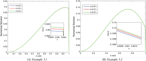
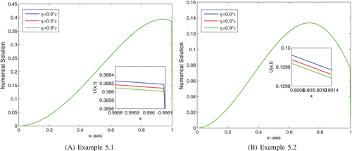
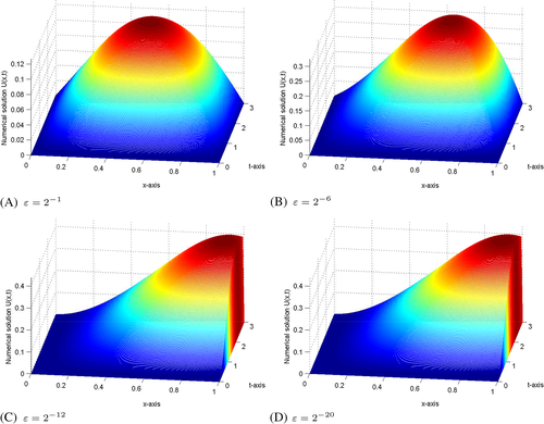
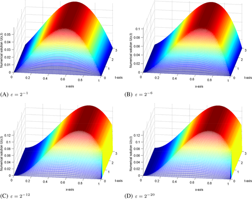
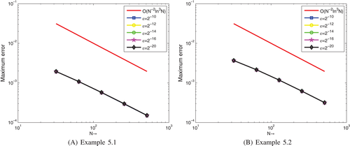
The effects of the $δ$ (negative shift) and $η$ (positive shift) are shown in Figures 1(A,B) and 2(A,B) on the solution profiles for Examples 1 and 2. From these figures, we can observe that as the size of $δ$ increases, the thickness of the layer increases (see Figure 1(A,B)), whereas as the size of $η$ increases, the thickness of the layer decreases (see Figure 2(A,B)). The 3D view of the numerical solution profiles for Examples 1 and 2 are displayed in Figures 3 and 4, respectively for $ε = 2^{- 1}, ε = 2^{- 6}, ε = 2^{- 12}$ , and $ε = 2^{- 20}$ . As it can be observed in Figures 3 and 4 as $ε \to 0$ a strong boundary layer is formed near $x = 1$ . In Figure 5(A,B), we have plotted a log-log plot of the $E_{ε, δ, η}^{N, M}$ verses N for Examples 1 and 2, respectively. As observed in Figure 5(A,B) the scheme in (25) is an $ε$ -uniformly convergent and stable.

Details are in the caption following the image — **FIGURE 1**
Open in figure viewer PowerPoint

Effect of $δ$ on the solution profile for $T = 3, ε = 2^{- 10}, η = 0.5 \times ε$

6 CONCLUSIONS

The robust numerical scheme is presented to solve the SPPDDEs arising in the modeling of neuronal variability. The scheme is proved to be an $ε$ -uniformly convergent accuracy of order $O (Λ t + N^{- 2} \ln^{3} N)$ . The efficiency of the scheme is shown by taking two test examples and comparing them with the numerical results in References 4, 7, 8. Concisely, the presented scheme is simple, stable and provides more accurate numerical results than the others.

ACKNOWLEDGMENT

The authors are grateful to the anonymous referees and editor for their constructive comments that will improve the quality of this manuscript.

CONFLICTS OF INTEREST

The authors declare that they have no competing interests.

Biographies

Imiru Takele Daba received his M.Sc. from Haramaya University, Ethiopia and Ph.D. scholar at Wollega University, Department of Mathematics, College of Natural and Computational Sciences, Ethiopia. His research interests include numerical methods for singularly perturbed differential-difference equations. He has published four research article in international reputable journal.
Gemechis File Duressa received his M.Sc. from Addis Ababa University, Ethiopia and Ph.D. from National Institute of Technology, Warangal, India. He is currently working as an associate professor at Jimma University, Ethiopia. His research interests include numerical methods for singularly perturbed differential equations, differential equations in ODE and PDE. He has published more than 80 research articles in various international reputable journals.

REFERENCES

1Stein RB. Some models of neuronal variability. Biophys J. 1967; 7(1): 37-68.
10.1016/S0006-3495(67)86574-3
CAS PubMed Web of Science® Google Scholar
2Musila M, Lánskỳ P. Generalized Stein's model for anatomically complex neurons. Biosystems. 1991; 25(3): 179-191.
10.1016/0303-2647(91)90004-5
CAS PubMed Web of Science® Google Scholar
3Ramesh V, Kadalbajoo MK. Upwind and midpoint upwind difference methods for time-dependent differential difference equations with layer behavior. Appl Math Comput. 2008; 202(2): 453-471.
10.1016/j.amc.2007.11.033
Web of Science® Google Scholar
4Kumar D, Kadalbajoo MK. A parameter-uniform numerical method for time-dependent singularly perturbed differential-difference equations. Appl Math Model. 2011; 35(6): 2805-2819.
10.1016/j.apm.2010.11.074
Web of Science® Google Scholar
5Bansal K, Rai P, Sharma KK. Numerical treatment for the class of time dependent singularly perturbed parabolic problems with general shift arguments. Differ Equ Dyn Syst. 2017; 25(2): 327-346.
10.1007/s12591-015-0265-7
Web of Science® Google Scholar
6Kumar D. An implicit scheme for singularly perturbed parabolic problem with retarded terms arising in computational neuroscience. Numer Methods Part Differ Equ. 2018; 34(6): 1933-1952.
10.1002/num.22269
Web of Science® Google Scholar
7Rao RN, Chakravarthy PP. Fitted numerical methods for singularly perturbed one-dimensional parabolic partial differential equations with small shifts arising in the modelling of neuronal variability. Differ Equ Dyn Syst. 2019; 27(1-3): 1-18.
10.1007/s12591-017-0363-9
Web of Science® Google Scholar
8Woldaregay MM, Duressa GF. Parameter uniform numerical method for singularly perturbed parabolic differential difference equations. J Nigerian Math Soc. 2019; 38(2): 223-245.
Google Scholar
9 Daba IT, Duressa GF. Extended cubic B-spline collocation method for singularly perturbed parabolic differential-difference equation arising in computational neuroscience. Int J Numer Methods Biomed Eng. 2020;e3418.
PubMed Web of Science® Google Scholar
10 Ramesh V, Priyanga B. Higher order uniformly convergent numerical algorithm for time-dependent singularly perturbed differential-difference equations. Differ Equ Dyn Syst. 2021; 29(1): 239-263.
10.1007/s12591-019-00452-4
Web of Science® Google Scholar
11Woldaregay MM, Duressa GF. Uniformly convergent numerical scheme for singularly perturbed parabolic delay differential equations. ITM Web Conf. 2020; 34(02011): 1-19.
Google Scholar
12 Daba IT, Duressa GF. A robust computational method for singularly perturbed delay parabolic convection-diffusion equations arising in the modelling of neuronal variability. Comput Methods Differ Equ. 2021.
Google Scholar
13 Govindarao L, Mohapatra J. Numerical analysis and simulation of delay parabolic partial differential equation involving a small parameter. Eng Comput. 2019.
Google Scholar
14Govindarao L, Mohapatra J, Das A. A fourth-order numerical scheme for singularly perturbed delay parabolic problem arising in population dynamics. J Appl Math Comput. 2020; 63(1): 171-195.
10.1007/s12190-019-01313-7
Web of Science® Google Scholar
15Shakti D, Mohapatra J. Numerical simulation and convergence analysis for a system of nonlinear singularly perturbed differential equations arising in population dynamics. J Differ Equ Appl. 2018; 24(7): 1185-1196.
10.1080/10236198.2018.1468891
Web of Science® Google Scholar
16Das A, Natesan S. Second-order uniformly convergent numerical method for singularly perturbed delay parabolic partial differential equations. Int J Comput Math. 2018; 95(3): 490-510.
10.1080/00207160.2017.1290439
Web of Science® Google Scholar
17Mekonnen TB, Duressa GF. Computational method for singularly perturbed two-parameter parabolic convection-diffusion problems. Cogent Math Stat. 2020; 7(1): 1829277.
10.1080/25742558.2020.1829277
Web of Science® Google Scholar
18 Mekonnen TB, Duressa GF. Uniformly convergent numerical method for two-parametric singularly perturbed parabolic convection-diffusion problems. J Appl Comput Mech. 2020.
Web of Science® Google Scholar
19Bullo TA, Duressa GF, Degla GA. Robust finite difference method for singularly perturbed two-parameter parabolic convection-diffusion problems. Int J Comput Methods. 2021; 18(2): 2050034.
10.1142/S0219876220500346
Web of Science® Google Scholar
20Tian H. The exponential asymptotic stability of singularly perturbed delay differential equations with a bounded lag. J Math Anal Appl. 2002; 270(1): 143-149.
10.1016/S0022-247X(02)00056-2
Web of Science® Google Scholar
21 Elsgolts LE, Norkin SB. Introduction to the Theory and Application of Differential Equations with Deviating Arguments. London: Elsevier; 1973.
Google Scholar
22Mohapatra J, Natesan S. The parameter-robust numerical method based on defect-correction technique for singularly perturbed delay differential equations with layer behavior. Int J Comput Methods. 2010; 7(04): 573-594.
10.1142/S0219876210002374
Web of Science® Google Scholar
23Sirisha L, Phaneendra K, Reddy YN. Mixed finite difference method for singularly perturbed differential difference equations with mixed shifts via domain decomposition. Ain Shams Eng J. 2018; 9(4): 647-654.
10.1016/j.asej.2016.03.009
Web of Science® Google Scholar
24Ladyzhenskaia OA, Solonnikov VA, Ural'tseva NN. Linear and Quasi-Linear Equations of Parabolic Type. Vol 23. Providence, RI: American Mathematical Society; 1968.
10.1090/mmono/023
Google Scholar
25Aziz T, Khan A. A spline method for second-order singularly perturbed boundary-value problems. J Comput Appl Math. 2002; 147(2): 445-452.
10.1016/S0377-0427(02)00479-X
Web of Science® Google Scholar

Citing Literature

All articles

A hybrid numerical scheme for singularly perturbed parabolic differential-difference equations arising in the modeling of neuronal variability

Abstract

1 INTRODUCTION

2 CONTINUOUS PROBLEM

3 DESCRIPTION OF THE NUMERICAL SCHEME

3.1 Temporal discretization

3.2 Spatial discretization

3.2.1 Hybrid numerical scheme

4 ERROR ANALYSIS

5 NUMERICAL EXAMPLES AND RESULTS

6 CONCLUSIONS

ACKNOWLEDGMENT

CONFLICTS OF INTEREST

Biographies

REFERENCES

Citing Literature

Figures

References

Information

About Wiley Online Library

Help & Support

Opportunities

Connect with Wiley

A hybrid numerical scheme for singularly perturbed parabolic differential-difference equations arising in the modeling of neuronal variability

Abstract

1 INTRODUCTION

2 CONTINUOUS PROBLEM

3 DESCRIPTION OF THE NUMERICAL SCHEME

3.1 Temporal discretization

3.2 Spatial discretization

3.2.1 Hybrid numerical scheme

4 ERROR ANALYSIS

5 NUMERICAL EXAMPLES AND RESULTS

6 CONCLUSIONS

ACKNOWLEDGMENT

CONFLICTS OF INTEREST

Biographies

REFERENCES

Citing Literature

Figures

References

Related

Information